Deploying a driving VLA: the onboard latency budget
Where the milliseconds go in a driving VLA and how to cut them: fewer image tokens, on-demand reasoning, fewer action steps, smaller weights, and hiding latency.
Why this matters
A driving model is not judged only on accuracy. It has to answer inside a deadline, every time, on hardware that fits in a car. The Alpamayo-R1 paper (AR1, 2511.00088) treats this as a design constraint from the first page: its vision encoder is built "to produce as few tokens as possible", its trajectory decoder is chosen to be fast, and it reports 99 ms end to end against a real-time requirement it states as typically 100 ms.
This module is about spending that budget. It answers four questions:
- Where do the milliseconds of one inference go?
- Which stage is limited by arithmetic and which by memory?
- Which techniques cut which stage, and what does each cost in quality?
- How do you keep the car safe when the deadline is missed anyway?
Most of the techniques were introduced earlier. Here they are placed on a latency budget, so you can tell which one to reach for.
1. The budget: one inference, four stages
One AR1 inference runs four stages in sequence. The paper's runtime table (measured on an NVIDIA RTX 6000 Pro Blackwell; the paper also reports on-vehicle road tests at 99 ms, and we have not checked what compute was in the car) gives:
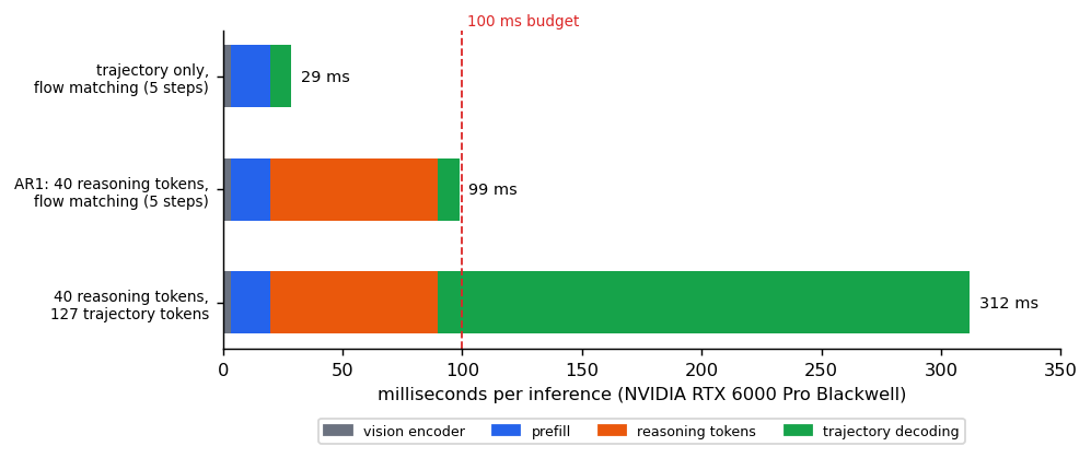
| Configuration | Vision encoder | Prefill | Reasoning decoding | Trajectory decoding | Total |
|---|---|---|---|---|---|
| Trajectory only, flow matching | 3.43 ms | 16.54 ms | none | 8.75 ms (5 steps) | 29 ms |
| AR1, flow matching | 3.43 ms | 16.54 ms | 70 ms (40 tokens) | 8.75 ms (5 steps) | 99 ms |
| AR1, autoregressive trajectory | 3.43 ms | 16.54 ms | 70 ms (40 tokens) | 222 ms (127 tokens) | 312 ms |
Three things follow from simple division, which is our arithmetic on the paper's numbers:
- A sequential step costs about the same wherever it happens. 70 ms over 40 reasoning tokens is 1.75 ms per token, 222 ms over 127 trajectory tokens is 1.75 ms per token, and 8.75 ms over 5 flow steps is 1.75 ms per step. The totals differ because the counts differ.
- Reasoning is about 70 percent of the full budget (70 of 99 ms). The trajectory-only model would use less than a third of the deadline.
- The vision encoder is nearly free here (3.43 ms) but its output is not. Its tokens set the prefill cost (16.54 ms) and sit in the KV cache for every later step (see Transformers).
A deadline applies to the slowest inference you will see, not the average. The paper reports one latency figure and does not say how it varies, so for your own system, measure the distribution (median and 99th percentile, after warm-up, on the target hardware, at realistic sequence lengths) and design for the tail.
2. What limits each stage
Two different bottlenecks matter:
- Prefill is limited by arithmetic. All prompt tokens are processed in parallel, so each weight loaded from memory is reused many times. More tokens means more computation, roughly in proportion.
- Decoding one token at a time is limited by memory. Each new token needs every weight once and does little arithmetic with it, so a step cannot be faster than the time to read the weights:
This is a lower bound for a batch of one. It ignores the KV cache, activations and launch overhead, so real steps are slower. With an illustrative 7-billion-weight model and a memory system of 1000 GB/s (hypothetical numbers, chosen for round arithmetic):
| Weights stored as | Bytes per weight | Lower bound per token |
|---|---|---|
| bf16 | 2 | 14 ms |
| int8 | 1 | 7 ms |
| 4-bit | 0.5 | 3.5 ms |
This is why quantization speeds up decoding: fewer bytes cross the memory bus. The paper does not state the precision, runtime or parallelism behind its 1.75 ms per token, so we do not try to reproduce that number from first principles. Do the same calculation for your own model and hardware before trusting any claimed speedup.
3. Fewer tokens in: compress the images
Every image token costs time in the vision encoder, prefill and the KV cache. A frame set from several cameras over several timesteps is a lot of tokens, so AR1's designers compress them. The paper's comparison of vision encoders, with the relative change in minADE₆ against a baseline of 160 tokens per image (negative is better):
| Method | Added parameters | Tokens per image | Change in minADE₆ |
|---|---|---|---|
| Baseline (single-image patches) | 0 | 160 | 0% |
| Triplane | 6.3M | 104 (1.5× fewer) | −3% |
| Triplane | 6.3M | 45 (3.6× fewer) | +4% |
| Flex (learned queries over all cameras and timesteps) | 61.6M | 50 (3.2× fewer) | −3% |
| Flex | 61.6M | 32 (5.0× fewer) | −3% |
| Flex | 61.6M | 16 (10× fewer) | −2% |
| Flex | 61.6M | 8 (20× fewer) | −2% |
The paper reports up to 20 times compression "while maintaining or even improving" driving metrics for the learned-query design. Read the numbers as one dataset and one metric: they do not show that nothing was lost in rare cases. The key idea, a small fixed set of query vectors that cross-attend to many images, is the object-query trick that also appears in perceivers and DETR.
Two further routes act on a model that is already trained:
- Token merging (ToMe, 2210.09461) combines similar tokens inside a ViT; the authors report roughly doubling throughput on large image models with a 0.2 to 0.3 percent accuracy drop, without retraining.
- Token pruning inside the language model: FastV (2403.06764) prunes visual tokens after an early layer and reports about 45 percent fewer FLOPs on LLaVA-1.5-13B at maintained performance. AR1 names post-training pruning (SparseVILA) as a path to larger backbones.
A toy that shows where pruning is safe
The reference code prunes the image tokens of the tiny VLM from the Tokens, ViT and VLMs module, which answers a colour question about a 16-token image. It prunes at two places and with two kinds of score:
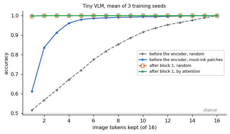
Over three seeds (uv run --group tutorial python scripts/tutorial_results.py deployment):
| Tokens kept of 16 | Before the encoder, random | Before the encoder, most non-zero pixels | After block 1, random | After block 1, by attention |
|---|---|---|---|---|
| 1 | 0.52 | 0.61 | 1.00 | 1.00 |
| 4 | 0.67 | 0.96 | 1.00 | 1.00 |
| 8 | 0.85 | 0.99 | 1.00 | 1.00 |
- Pruning before the encoder throws information away. A random patch is often background, and the answer needs both squares. Choosing patches by content is much better but still loses accuracy when very few remain. Its saving is the largest, because the encoder and everything after it see fewer tokens.
- Pruning after a block that has already read the image loses nothing here. The answer token attended to every image token in block 1, so the information has moved; the remaining image tokens are dead weight. This is the idea behind FastV: its title says "after layer 2". The saving is smaller, because the first layers still ran on every token.
- The toy is too easy to say how much to prune. Its first block moves everything it needs, and random pruning after it does as well as attention-based pruning. In a real model the information moves gradually over many layers, the score matters, and you must measure driving metrics, not toy accuracy.
4. Fewer tokens out: reason only when it pays
Reasoning is the biggest block in AR1's budget (section 1). The paper's own future-work section points at the fix: reasoning on demand, invoking reasoning "only for safety-critical or ambiguous scenarios" rather than for every input. AutoVLA (2506.13757) trains this directly: its abstract describes a fast (trajectory-only) and a slow (step-by-step reasoning) mode, and a GRPO-based fine-tuning step meant to cut reasoning that is not needed in simple situations.
With AR1's numbers the mean latency, if reasoning runs on a fraction of the inputs, is:
| Share of inputs that reason | Mean latency |
|---|---|
| 0% | 28.7 ms |
| 10% | 35.7 ms |
| 25% | 46.2 ms |
| 50% | 63.7 ms |
| 100% | 98.7 ms |
Two cautions, both about the deadline rather than the mean:
- The slow path still takes about 99 ms. If the deadline is 100 ms, the system has gained throughput and compute headroom, not a smaller worst case. Whether that matters depends on whether the slow path may run late safely, which is a system-design question.
- The gate needs a signal. Something must decide which inputs deserve reasoning, and a wrong "this is easy" is exactly the failure that matters. The gate is a good place for the uncertainty tools in Uncertainty and runtime safety.
Other ways to spend fewer decoding steps: shorter, more concise reasoning traces; speculative decoding (see Efficient fine-tuning and inference); and early exit. DeeR-VLA (2411.02359) stops a robot VLA's language model at an earlier layer when the situation allows, and reports 5.2 to 6.5 times less LLM computation on the CALVIN benchmark (a manipulation benchmark, not driving).
5. Fewer action steps
AR1 decodes the trajectory with a flow-matching action expert in 5 steps (8.75 ms) rather than as 127 text tokens (222 ms). The saving comes from the structure in section 1: cost is the number of sequential steps times the cost of one. The Flow matching and Sampling and guidance modules show why few steps can work for a smooth, low-dimensional output, and measure it on a toy.
Chunking amortises the rest. One inference produces a whole chunk of future waypoints that the controller follows over many ticks (see Imitation learning and action chunking), so, for example, the model can run at 10 Hz while the controller runs faster. OpenVLA-OFT (2502.19645) combines parallel decoding, chunking, continuous actions and an L1 objective and reports 26 times higher action-generation throughput (on the LIBERO benchmark, where it also raised success from 76.5 to 97.1 percent).
6. Smaller weights: quantization in practice
Section 2 says decoding is limited by bytes read, so fewer bits per weight is the most direct fix. The int8 reference in Efficient fine-tuning and inference shows the mechanism. Two methods matter at LLM scale:
- SmoothQuant (2211.10438) quantizes both weights and activations to 8 bits. Activations have large outliers that are hard to quantize, so it moves that difficulty into the weights with a mathematically equivalent rescaling.
- AWQ (2306.00978) quantizes weights only, to low bit widths, protecting the small share of channels that activation statistics mark as important; it targets edge devices.
Three practical points for a driving model:
- Re-run the driving evaluation after quantizing. An average metric can hide a loss on rare events, and rare events are the point of a safety-critical model. This is our advice, not a measured result; the papers above evaluate language and robot benchmarks.
- Use calibration data that includes the long tail, because the scale factors are fitted on it.
- Quantize the parts that dominate the budget. The vision encoder is 3.43 ms of the 99; the backbone's decode steps are most of the rest.
7. Hiding latency: asynchronous execution
If an inference takes 100 ms, a robot that waits for each result before moving is idle part of the time, and a car cannot wait at all. The fix is to overlap them: start the next inference while the current chunk is still being followed.
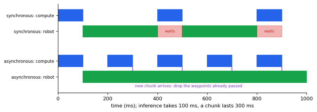
One thing must change when you do this: the plan is old when it arrives. It was computed from
the world at time 0 and describes waypoints for 0, 0.1 s, 0.2 s and so on. If inference took 200 ms,
the vehicle is already 200 ms into that plan, so the first two waypoints are in the past and must be
skipped, not driven. The plan is also written relative to where the car was at time 0, so it must be
re-expressed in the car's current frame. drop_elapsed in the reference code does the first part.
SmolVLA (2506.01844) builds an asynchronous inference stack that separates prediction from execution, for responsiveness and higher control rates (see also the VLA models module). Real-time chunking (2506.07339) goes further for diffusion and flow policies: it plans the next chunk while the current one runs, keeps the actions already committed and regenerates the rest, without retraining, so chunk boundaries stay smooth.
8. When the deadline is missed anyway
Some inference will be late, because of a slow frame, a thermal limit or contention. The system around the model needs a rule for that, decided in advance:
- A watchdog that notices a missing result by the deadline, rather than waiting for it.
- Keep driving the last plan while its remaining waypoints are valid (this is what
drop_elapsedimplies: the plan has a horizon), and when it runs out, hand over to a fallback: a simple, non-learned planner or a minimal-risk manoeuvre. - Log latency percentiles and every miss, so that you notice drift before it matters.
This is the same pattern as the runtime monitor in Uncertainty and runtime safety: the learned model proposes, and a simpler component with a guarantee decides what is allowed.
Which technique for which stage
| Technique | Cuts | Costs |
|---|---|---|
| Fewer, learned image tokens | Vision encoder, prefill, KV cache | Retraining; possible loss of detail |
| Post-hoc token merging or pruning | Prefill (and later steps) | Quality loss if the score is poor; needs measuring |
| Reasoning on demand | Decoding steps on most inputs | A gate that can be wrong; worst case unchanged |
| Flow matching in few steps | Action decoding | Quality at very low step counts; a separate action expert |
| Weight quantization | Every decoding step | Possible loss on rare cases; calibration effort |
| Asynchronous execution | Idle time and perceived delay | Stale plans: must drop elapsed waypoints and re-frame |
| Watchdog and fallback | Risk of a missed deadline | A second planner to build and verify |
Reference implementation (PyTorch)
libs/tutorial/deployment.py has a latency profile that reproduces the paper's totals, the
memory-bound lower bound, token pruning at two places on the tiny VLM, and drop_elapsed. Tests are
in libs/tutorial/tests/test_deployment.py: the profile gives 99, 29 and 312 ms from the paper's
per-stage numbers, expected latency interpolates between the fast and slow paths, halving the bytes
halves the memory-bound time, a late plan loses exactly its elapsed waypoints, keeping every token
changes nothing, content-aware pruning before the encoder beats random pruning, and pruning after
the first block loses almost nothing. Run uv run --group tutorial python -m libs.tutorial.deployment.
@dataclass(frozen=True)
class LatencyProfile:
    """Per-stage costs of one inference, in milliseconds.

    Attributes:
        vision_ms: Vision encoder time for one frame set.
        prefill_ms: Time to run the prompt (image tokens, route) through the backbone.
        ms_per_reasoning_token: Cost of one autoregressive step of the backbone.
        ms_per_action_step: Cost of one denoising step of the action decoder.
    """

    vision_ms: float
    prefill_ms: float
    ms_per_reasoning_token: float
    ms_per_action_step: float

    def total_ms(self, reasoning_tokens: int, action_steps: int) -> float:
        """Latency of one inference producing the given number of tokens and steps.

        Raises:
            ValueError: If a count is negative.
        """
        if reasoning_tokens < 0 or action_steps < 0:
            raise ValueError(
                f"counts must be non-negative, got {reasoning_tokens} tokens and "
                f"{action_steps} steps"
            )
        return (
            self.vision_ms
            + self.prefill_ms
            + reasoning_tokens * self.ms_per_reasoning_token
            + action_steps * self.ms_per_action_step
        )

    def expected_ms(
        self, reason_fraction: float, reasoning_tokens: int, action_steps: int
    ) -> float:
        """Mean latency when reasoning runs on only a fraction of the inputs.

        Raises:
            ValueError: If ``reason_fraction`` is outside [0, 1].
        """
        if not 0.0 <= reason_fraction <= 1.0:
            raise ValueError(
                f"reason_fraction must be in [0, 1], got {reason_fraction}"
            )
        return self.total_ms(0, action_steps) + reason_fraction * (
            self.total_ms(reasoning_tokens, action_steps)
            - self.total_ms(0, action_steps)
)def memory_bound_ms_per_token(
parameters: float, bytes_per_parameter: float, bandwidth_gb_per_s: float
) -> float:
"""Lower bound on one decoding step when weight reads are the bottleneck.
With a batch of one, each new token needs every weight once and does very little
arithmetic with it, so the step takes at least (bytes of weights) / (memory
bandwidth). This ignores the KV cache, activations and launch overheads, so real
steps are slower.
Args:
parameters: Number of weights read per token.
bytes_per_parameter: 2 for bf16, 1 for int8, 0.5 for 4-bit.
bandwidth_gb_per_s: Memory bandwidth in gigabytes (1e9 bytes) per second.
Raises:
ValueError: If bandwidth is not positive.
"""
if bandwidth_gb_per_s <= 0:
raise ValueError(f"bandwidth must be positive, got {bandwidth_gb_per_s}")
return parameters * bytes_per_parameter / (bandwidth_gb_per_s * 1e9) * 1e3def _language_tokens(
model: TinyVLM, image_tokens: torch.Tensor, questions: torch.Tensor
) -> torch.Tensor:
"""Appends the question token and the answer slot to projected image tokens."""
text = model.question(questions)[:, None]
slot = model.answer_slot.expand(len(image_tokens), -1, -1)
return torch.cat([image_tokens, text, slot], dim=1)
def _top_indices(scores: torch.Tensor, keep: int) -> torch.Tensor:
"""Indices of the ``keep`` highest scores per row, in their original order."""
if not 1 <= keep <= scores.shape[1]:
raise ValueError(f"keep must be in [1, {scores.shape[1]}], got {keep}")
return scores.topk(keep, dim=1).indices.sort(dim=1).values
@torch.no_grad()
def input_pruned_logits(
model: TinyVLM,
images: torch.Tensor,
questions: torch.Tensor,
keep: int,
score: str = "random",
) -> torch.Tensor:
"""Keeps only ``keep`` image patches before the vision encoder runs.
Cheap, because the encoder and everything after it see fewer tokens, but the
discarded patches are gone for good. ``"energy"`` keeps the patches with the most
non-zero pixels; ``"random"`` ignores the content.
Raises:
ValueError: If ``keep`` is out of range or ``score`` is unknown.
"""
if score not in ("random", "energy"):
raise ValueError(f"score must be 'random' or 'energy', got {score!r}")
vision = model.vision
embedded = vision.patches(images) + vision.position
if score == "energy":
scores = patchify(images, vision.patches.proj.kernel_size[0]).abs().sum(dim=-1)
else:
scores = torch.rand(len(images), embedded.shape[1])
rows = torch.arange(len(images))[:, None]
tokens = embedded[rows, _top_indices(scores, keep)]
for block in vision.blocks:
tokens = block(tokens)
image_tokens = model.projector(vision.norm(tokens))
tokens = _language_tokens(model, image_tokens, questions)
for block in model.blocks:
tokens = block(tokens)
return model.head(model.norm(tokens[:, -1]))
@torch.no_grad()
def block_pruned_logits(
model: TinyVLM,
images: torch.Tensor,
questions: torch.Tensor,
keep: int,
score: str = "attention",
) -> torch.Tensor:
"""Keeps only ``keep`` image tokens after the language model's first block.
The first block sees every token, so information has already moved from the image
tokens into the question and answer tokens. ``"attention"`` keeps the tokens the
answer slot attended to most in that block (the idea of FastV); ``"random"``
ignores the scores.
Raises:
ValueError: If ``keep`` is out of range or ``score`` is unknown.
"""
if score not in ("random", "attention"):
raise ValueError(f"score must be 'random' or 'attention', got {score!r}")
image_tokens = model.projector(model.vision(images))
tokens = _language_tokens(model, image_tokens, questions)
first, *rest = model.blocks
if score == "attention":
weights = first.attn.attention_weights(first.norm1(tokens))
scores = weights[:, :, -1, :PATCHES].mean(dim=1)
else:
scores = torch.rand(len(images), PATCHES)
kept = _top_indices(scores, keep)
tokens = first(tokens)
rows = torch.arange(len(images))[:, None]
tokens = torch.cat([tokens[rows, kept], tokens[:, PATCHES:]], dim=1)
for block in rest:
tokens = block(tokens)
return model.head(model.norm(tokens[:, -1]))def drop_elapsed(plan: torch.Tensor, latency_s: float, dt: float) -> torch.Tensor:
"""Discards the part of a plan that is already in the past when it arrives.
A planner reads the world at time 0 and returns waypoints for 0, dt, 2 dt, ...
If inference took ``latency_s``, the vehicle is already ``latency_s`` into that
plan, so the first ``ceil(latency_s / dt)`` waypoints must be skipped, not driven.
Args:
plan: Waypoints of shape (n, 2), one per ``dt``.
latency_s: Time from reading the world to having the plan.
dt: Spacing of the waypoints in seconds.
Raises:
ValueError: If ``latency_s`` is negative, ``dt`` is not positive, or the plan
is shorter than the latency.
"""
if latency_s < 0 or dt <= 0:
raise ValueError(f"need latency_s >= 0 and dt > 0, got {latency_s}, {dt}")
skip = math.ceil(latency_s / dt - 1e-9)
if skip >= len(plan):
raise ValueError(f"plan of {len(plan)} waypoints is shorter than {latency_s} s")
return plan[skip:]Check yourself
- In AR1's runtime table, which stage is the largest share of the 99 ms, and how much?
- Why can a batch-of-one decoding step not be faster than (weight bytes) / (memory bandwidth)?
- If reasoning runs on a quarter of the inputs, what happens to the mean latency and to the worst case?
- Why did pruning after the first block cost the toy nothing, while pruning before the encoder did?
- A plan arrives 300 ms after the observation, with waypoints every 100 ms. What do you do with the first three?
Answers
- Decoding the reasoning tokens: 70 ms of 99 ms, about 71 percent.
- Each decoding step must read every weight from memory once, and at batch size one there is little arithmetic per byte read, so the step cannot finish faster than the time to move the weights.
- The mean falls from about 99 ms to about 46 ms. The worst case does not change: an input that reasons still takes about 99 ms.
- In the tiny VLM the answer slot attends to every image token in the first block, so later blocks no longer need most of them. Pruning before the encoder removes information that was never read.
- Drop them: they describe where the car should have been 100, 200 and 300 ms ago. Execute from the fourth, re-expressed in the car's current frame.
Quiz
Answer each question; feedback appears as soon as you choose.
Sources
- NVIDIA et al., Alpamayo-R1, 2025: runtime table, vision-encoder comparison, reasoning on demand.
- Zhou et al., AutoVLA, 2025.
- Yue et al., DeeR-VLA, 2024.
- Kim et al., Fine-Tuning Vision-Language-Action Models: Optimizing Speed and Success, 2025.
- Black et al., Real-Time Execution of Action Chunking Flow Policies, 2025.
- Bolya et al., Token Merging: Your ViT But Faster, 2022.
- Chen et al., An Image is Worth 1/2 Tokens After Layer 2, 2024 (FastV).
- Xiao et al., SmoothQuant, 2022.
- Lin et al., AWQ, 2023.
- Shukor et al., SmolVLA, 2025.
Efficient fine-tuning and inference
Adapting and serving large models on small hardware: LoRA and QLoRA, quantization in depth (scales, groups, outliers, int8 and 4-bit), the KV cache, FlashAttention's online softmax, speculative decoding and distillation.
From modular stacks to end-to-end driving
For engineers who built perception, prediction and planning modules: what end-to-end learning replaces, what it keeps, where hand-designed interfaces lose information, and how hybrid stacks combine both.