Transformers

The problem

Many inputs are sets or sequences of variable length in which any element may depend on any other: words in a sentence, patches in an image, camera frames, waypoints. The usual architectures each struggle with this in a different way.

An MLP wants a fixed-size input. Its first layer is a matrix with one column per input number, so its shape is tied to the input length:

• Different lengths do not fit. A flattened 10-token sequence and a 1,000-token sequence need different matrices, so you must pad or truncate.
• Parameters grow with the input. Flatten 1,000 tokens of 512 features each and the layer sees 512,000 numbers. Feeding them into a 2,048-wide hidden layer takes 512,000 x 2,048, about 1.05 billion weights, in that first layer alone.
• Nothing is shared across positions. The weights that read position 3 are separate from those that read position 7, so a pattern learned at one position has to be relearned at every other.

A CNN shares weights across positions but only looks at neighbours, so a distant pair of elements interacts only after many layers. A recurrent network accepts any length but must walk through the tokens one at a time.

A transformer applies the same weights to every token. The query, key and value projections and the MLP in a block act on one token at a time, with the same matrices for each. A block has about 3.15 million parameters at width 512 (counting biases and layer norms) whether the sequence has 10 tokens or 1,000, because the sequence length is a dimension of the data, not of the parameters. Attention then lets any token read any other through an n by n table of scores built from those shared projections, with no weight per pair of positions.

It is not unlimited. A table of learned position vectors has a maximum length, sinusoidal or rotary positions extend further but quality falls beyond the lengths seen in training, and attention cost grows with the square of the length (see Cost below).

This module builds the transformer in the order a forward pass meets its parts. For a second telling with different pictures, read Jay Alammar's The Illustrated Transformer alongside it (see the end of this page for what each resource adds).

Three shapes of transformer

The 2017 paper introduced one design, an encoder stack feeding a decoder stack, for machine translation. Its sizes are a useful reference: six layers in each stack, model width 512, 8 attention heads, 64 features per head. Today the same parts are used in three arrangements:

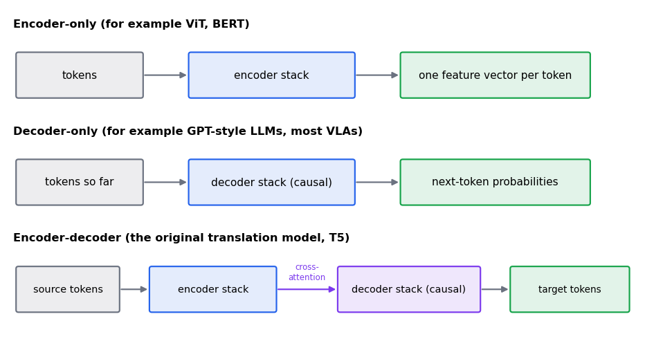
Everything below applies to all three. The differences are two switches: whether attention is masked (decoders only look backwards) and whether a layer cross-attends to another sequence (encoder-decoder only).

From tokens to vectors

Text becomes token ids, and an embedding table turns each id into a vector (the Tokens, ViT and VLMs module). Images become patch vectors the same way. From here on a transformer sees only a matrix X of shape (n, d): one row per token. Each row travels through the stack in its own lane, and attention is the only place where lanes talk to each other. The MLP in each block, by contrast, treats every row separately, which is why the whole sequence can be processed in parallel.

Self-attention step by step

Take a sequence of n vectors, stacked as a matrix X with shape (n, d).

1. Project. Make three linear projections: queries $Q = X W_q$, keys $K = X W_k$, values $V = X W_v$. A useful reading: the query is what a token is looking for, the key is what it offers to be found by, and the value is what it passes on if it is chosen.
2. Score. $S = Q K^\top / \sqrt{d_k}$, shape (n, n). Entry (i, j) is how relevant token j is to token i. The division by $\sqrt{d_k}$ keeps scores from growing with dimension, which would make softmax saturate.
3. Normalise. Softmax each row, so the weights for token i sum to 1.
4. Mix. Output $\mathrm{softmax}(S)\,V$: each token becomes a weighted average of the values.

In one line:

$\mathrm{Attention}(Q,K,V) = \mathrm{softmax}\!\left(\frac{QK^\top}{\sqrt{d_k}}\right)V$

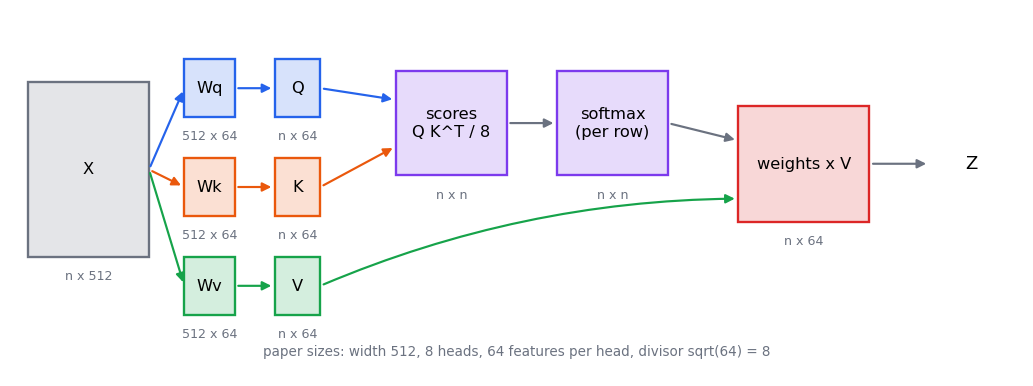
Think of it as a soft, learned lookup: a query compares itself with all keys and reads a mix of the matching values. Unlike a convolution, the weights depend on the content, not on fixed positions. Unlike a recurrent network, token 1 and token 500 are one step apart.

A worked example you can check by hand

Three tokens with two features: x1 = (1, 0), x2 = (0, 1), x3 = (1, 1). Take Wq = Wk = Wv = identity, so Q = K = V = X, and d_k = 2.

• Scores: $S = XX^\top/\sqrt{2}$ gives rows (0.707, 0, 0.707), (0, 0.707, 0.707) and (0.707, 0.707, 1.414).
• Softmax per row gives weights (0.401, 0.198, 0.401), (0.198, 0.401, 0.401) and (0.248, 0.248, 0.503).
• Outputs, the weighted sums of the values: (0.802, 0.599), (0.599, 0.802) and (0.752, 0.752).

Token 3 is similar to both others, so it attends to itself most and gets an even mix of x1 and x2. Token 1 attends equally to itself and to token 3, because they share the first feature.

Many heads

One attention gives each token one set of weights. Multi-head attention runs several attentions in parallel, each on its own smaller slice of the features, so different heads can look at different positions or relations. In the original sizes the 512 features become 8 heads of 64. Each head produces an (n, 64) output; the eight are concatenated back to (n, 512) and mixed by one more matrix $W_o$:

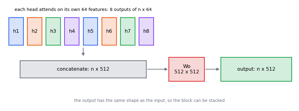
Because each head works on 64 features rather than 512, eight heads cost about the same as one big head. The reference code below does exactly this split with a reshape.

Telling the model where things are

Attention treats its input as a set: the exercise below shows that shuffling the rows only shuffles the outputs. So order has to be injected. The original paper adds a fixed position vector to each embedding. Entry $2i$ of the vector for position $p$ is a sine, and entry $2i+1$ is the matching cosine, at a different frequency for each $i$:

$\mathrm{PE}_{p,2i} = \sin\!\left(\frac{p}{10000^{2i/d}}\right), \qquad \mathrm{PE}_{p,2i+1} = \cos\!\left(\frac{p}{10000^{2i/d}}\right)$

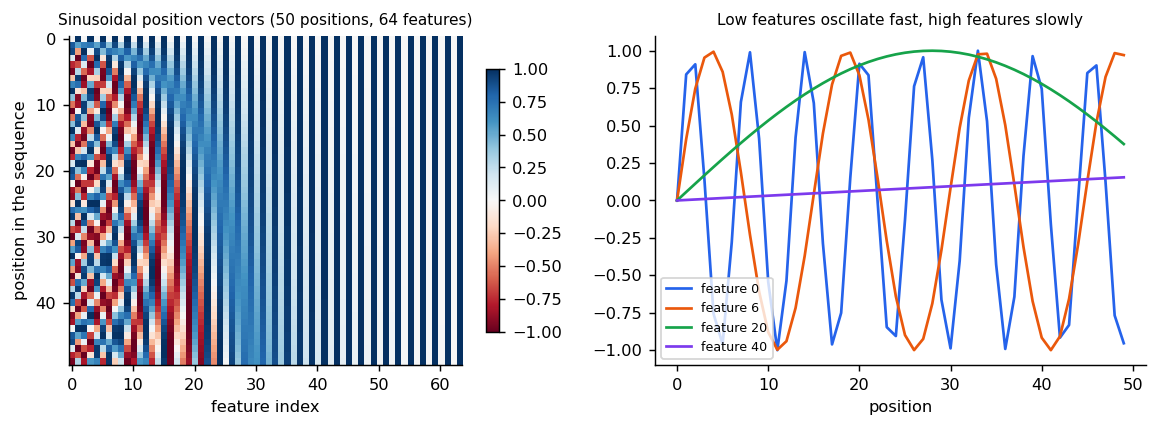
Other choices are common. Many models learn the position vectors instead. Others, such as RoFormer (2104.09864), apply a rotary position embedding that rotates queries and keys by an angle that depends on position, so attention scores depend on relative offsets. Whatever the scheme, without one the model cannot tell "the robot pushed the cube" from "the cube pushed the robot".

def sinusoidal_positions(length: int, dim: int) -> torch.Tensor:
    """Fixed sine and cosine position vectors from the original transformer paper.

    Entry (pos, 2i) is sin(pos / 10000^(2i/dim)) and entry (pos, 2i + 1) is the matching
    cosine, so every position gets a unique pattern and nearby positions look similar.

    Args:
        length: Number of positions.
        dim: Feature size; must be even.

    Returns:
        A tensor of shape (length, dim).

    Raises:
        ValueError: If ``dim`` is odd.
    """
    if dim % 2 != 0:
        raise ValueError(f"dim must be even, got {dim}")
    position = torch.arange(length, dtype=torch.float32)[:, None]
    frequency = torch.exp(-math.log(10000.0) * torch.arange(0, dim, 2) / dim)
    table = torch.zeros(length, dim)
    table[:, 0::2] = torch.sin(position * frequency)
    table[:, 1::2] = torch.cos(position * frequency)
    return table

The rest of the block

Attention is half of a transformer block. The other half and the glue:

• A position-wise MLP. The same two-layer network applied to every token separately, usually widening the features first (512 to 2048 and back in the original). Attention moves information between tokens; the MLP processes it within each token.
• Residual connections. Each sublayer's output is added to its input (see ResNet). The stack becomes a running "stream" that each layer reads from and writes to, and gradients have a direct path back through the additions.
• Layer normalisation. Features of each token are rescaled to zero mean and unit variance (Ba et al.), which keeps training stable. The original paper normalises after each residual addition (post-norm). Our reference block normalises before each sublayer (pre-norm), the common modern choice: Xiong et al. (2002.04745) report that pre-norm has well-behaved gradients at initialisation and removes the need for learning-rate warm-up, while post-norm produces large gradients near the output at initialisation.

Masks, cross-attention and decoding

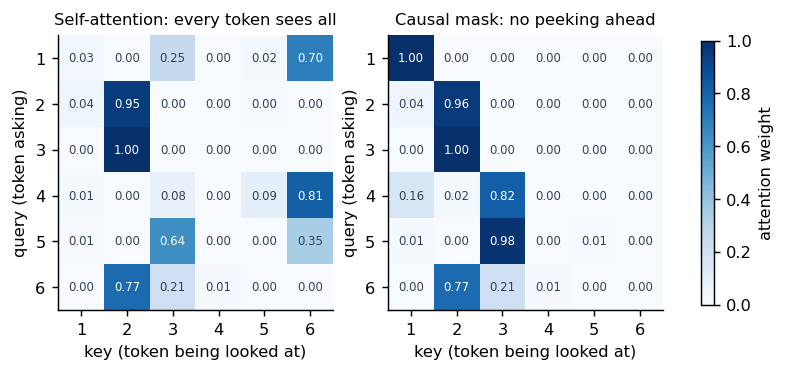
A decoder predicts the next token, so position i must not see tokens after it. A causal mask sets the scores for later positions to minus infinity before the softmax, so their weights become exactly zero. That is the right-hand heatmap above.

An encoder-decoder model adds a third sublayer to each decoder block: cross-attention. Its queries come from the decoder, but its keys and values come from the encoder's output, so each target token can look at the whole source. In the reference code, passing context to the attention layer is all it takes.

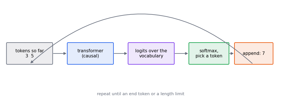
Generation is a loop. The model reads the tokens so far, a linear layer turns the last position's feature vector into one score per vocabulary item (the logits), softmax turns those into probabilities, one token is chosen, and the loop repeats with it appended:

Training: all positions at once

Training uses the same forward pass with a known target. For a decoder-only model the target at every position is simply the next token of the training text. With the causal mask, one pass predicts the next token at every position at once, and the loss is the average cross-entropy (the negative log of the probability given to the right token, from the Before you start page) over those positions. Feeding the true previous tokens rather than the model's own guesses during training is called teacher forcing. This parallelism is a large part of why transformers train so much faster than recurrent networks, which must process tokens one after another.

Generation without wasted work: the KV cache

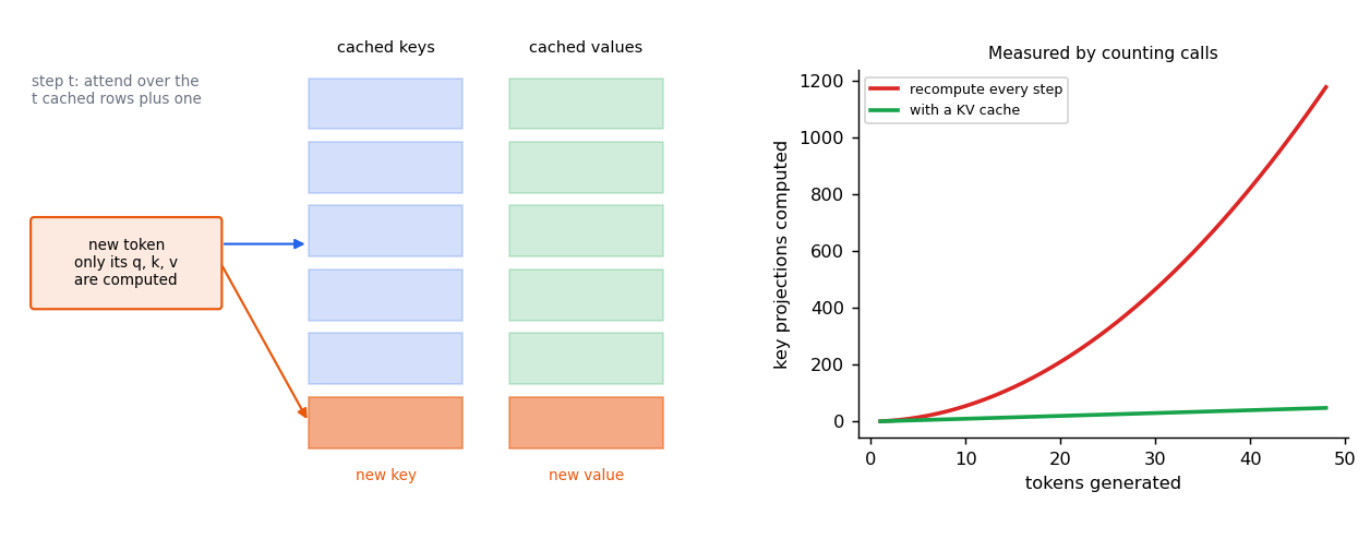
Generating text one token at a time looks wasteful. To produce token $t$ the model attends over tokens $1 \ldots t$, and a naive loop would rerun the whole network on the whole prefix at every step. But with a causal mask, an earlier token never sees a later one, so the keys and values of tokens $1 \ldots t-1$ do not change when token $t$ arrives. A key-value cache (KV cache) stores them, so each step computes the query, key and value of the new token only and attends over the stored keys and values plus its own.

The two kinds of work in generation have different characters:

• Prefill processes the whole prompt (including any image tokens) in one parallel pass and fills the cache. It is limited by arithmetic.
• Decode then adds one token per step. Each step does little arithmetic but must read the whole cache from memory, so it is typically limited by memory bandwidth, not by compute. Shazeer's multi-query attention paper (1911.02150) makes this point about incremental decoding.

The Alpamayo-R1 paper's latency table shows both stages: about 16.5 ms for prefilling and 70 ms to decode 40 reasoning tokens (the Driving VLA concepts page breaks down the 99 ms total). Its flow-matching action expert also reads the VLM's key-value cache instead of recomputing the prefix.

What it saves and what it costs

In our single-layer reference code, decoding 512 tokens passes 512 token rows through the key projection with the cache and 131,328 without it (n(n+1)/2). On one CPU the wall time was about 108 ms against 561 ms (median of 3 runs; the exact times depend on the machine, the counts do not; uv run --group tutorial python scripts/tutorial_results.py kv_cache reproduces both). The cache trades memory for compute, and the memory is not small. Every layer stores a key and a value for every cached token:

$\text{cache bytes} = 2 \times \text{layers} \times \text{KV heads} \times \text{head size} \times \text{tokens} \times \text{batch} \times \text{bytes per value}$

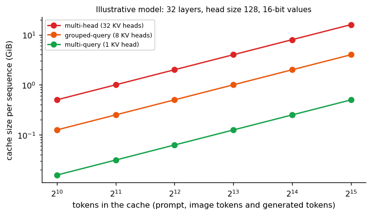
For an illustrative model with 32 layers, 32 heads of size 128 and 16-bit values, that is 0.5 MiB per token, so a 4,096-token sequence needs 2 GiB, and a prompt with 7,168 image tokens (seven cameras over four frames at 256 tokens each, as in the Tokens, ViT and VLMs page) needs 3.5 GiB before a single word is generated. This is a configuration chosen for arithmetic, not any particular model.

Shrinking the cache

• Share key-value heads. Multi-query attention (Shazeer, above) gives all query heads one set of keys and values, shrinking the tensors that must be read; he reports faster decoding with only a minor quality loss. Grouped-query attention (GQA, 2305.13245) uses a middle number of key-value heads, close to multi-head quality at multi-query speed, and the authors convert existing multi-head checkpoints with about 5 percent of the original pre-training compute.
• Manage the memory. PagedAttention (2309.06180) stores the cache in blocks so many requests can share a GPU without wasting space.
• Keep fewer tokens. Compress image tokens (SmolVLA keeps 64 per frame) or shorten generated reasoning, as the Reasoning module discusses.

@torch.no_grad()
def decode_with_cache(layer: MultiHeadAttention, tokens: torch.Tensor) -> torch.Tensor:
    """Runs causal self-attention one token at a time, reusing past keys and values.

    The result equals ``layer(tokens, causal=True)`` but each new token only computes
    its own query, key and value instead of recomputing every earlier one.

    Args:
        layer: A multi-head attention layer.
        tokens: Shape (batch, n, dim).

    Returns:
        Outputs of shape (batch, n, dim).
    """
    keys: list[torch.Tensor] = []
    values: list[torch.Tensor] = []
    outputs = []
    for position in range(tokens.shape[1]):
        new = tokens[:, position : position + 1]
        keys.append(layer.split(layer.k_proj(new)))
        values.append(layer.split(layer.v_proj(new)))
        q = layer.split(layer.q_proj(new))
        k, v = torch.cat(keys, dim=2), torch.cat(values, dim=2)
        weights = (q @ k.transpose(-2, -1) / math.sqrt(q.shape[-1])).softmax(dim=-1)
        out = (weights @ v).transpose(1, 2).reshape(len(tokens), 1, -1)
        outputs.append(layer.out_proj(out))
    return torch.cat(outputs, dim=1)

@torch.no_grad()
def decode_without_cache(
    layer: MultiHeadAttention, tokens: torch.Tensor
) -> torch.Tensor:
    """The same outputs as ``decode_with_cache``, recomputing the prefix every step."""
    outputs = [
        layer(tokens[:, : position + 1], causal=True)[:, -1:]
        for position in range(tokens.shape[1])
    ]
    return torch.cat(outputs, dim=1)


def kv_cache_bytes(
    layers: int,
    kv_heads: int,
    head_dim: int,
    seq_len: int,
    batch: int = 1,
    bytes_per_value: int = 2,
) -> int:
    """Memory needed to cache keys and values.

    Every layer stores one key and one value vector per cached token for each
    key-value head, so the total is 2 * layers * kv_heads * head_dim * seq_len * batch
    values of ``bytes_per_value`` bytes each (2 for fp16 or bf16).

    Args:
        layers: Number of transformer blocks.
        kv_heads: Number of key-value heads; equal to the query heads for multi-head
            attention, 1 for multi-query attention, in between for grouped-query.
        head_dim: Features per head.
        seq_len: Number of cached tokens (prompt, image tokens and generated tokens).
        batch: Number of sequences held at once.
        bytes_per_value: Bytes per stored number.
    """
    return 2 * layers * kv_heads * head_dim * seq_len * batch * bytes_per_value

Tests (libs/tutorial/tests/test_efficiency.py) check that cached and uncached decoding give the same outputs, that the key-projection counts are exactly $n$ and $n(n+1)/2$, and that the memory formula gives 2 GiB for the example, a quarter of it for 8 key-value heads and a thirty-second for one.

Put it together: a tiny GPT you can run

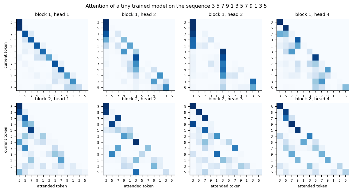
The reference code below assembles every piece above into a small decoder-only model: token embeddings plus sinusoidal positions, two causal blocks, a final layer norm and a vocabulary head. The toy task: each sequence is an arithmetic progression modulo 10 with a hidden step (3 5 7 9 1 3 ... has step 2; 8 1 4 7 0 ... has step 3). The first two tokens cannot be predicted, but after two tokens the step is determined, so the model has to look back, which is exactly what attention does.

class TinyGPT(nn.Module):
    """Token embeddings plus positions, causal blocks, then a vocabulary head."""

    def __init__(
        self, vocab: int = VOCAB, dim: int = 64, heads: int = 4, depth: int = 2
    ) -> None:
        """Creates the model.

        Args:
            vocab: Number of distinct tokens.
            dim: Feature size.
            heads: Attention heads per block.
            depth: Number of transformer blocks.
        """
        super().__init__()
        self.tokens = nn.Embedding(vocab, dim)
        self.register_buffer("positions", sinusoidal_positions(64, dim))
        self.blocks = nn.ModuleList(TransformerBlock(dim, heads) for _ in range(depth))
        self.norm = nn.LayerNorm(dim)
        self.head = nn.Linear(dim, vocab)

    def embed(self, ids: torch.Tensor) -> torch.Tensor:
        """Token embeddings plus position vectors, shape (batch, n, dim)."""
        return self.tokens(ids) + self.positions[: ids.shape[1]]

    def forward(self, ids: torch.Tensor) -> torch.Tensor:
        """Maps token ids (batch, n) to next-token logits (batch, n, vocab)."""
        x = self.embed(ids)
        for block in self.blocks:
            x = block(x, causal=True)
        return self.head(self.norm(x))

    @torch.no_grad()
    def attention_maps(self, ids: torch.Tensor) -> list[torch.Tensor]:
        """Attention weights (batch, heads, n, n) of every block for ``ids``."""
        maps = []
        x = self.embed(ids)
        for block in self.blocks:
            maps.append(block.attn.attention_weights(block.norm1(x), causal=True))
            x = block(x, causal=True)
        return maps

def next_token_loss(logits: torch.Tensor, ids: torch.Tensor) -> torch.Tensor:
    """Cross-entropy of predicting token t + 1 from tokens up to t."""
    return F.cross_entropy(logits[:, :-1].flatten(0, 1), ids[:, 1:].flatten())


@torch.no_grad()
def predictable_accuracy(model: TinyGPT, ids: torch.Tensor) -> float:
    """Share of next-token predictions that are right, from the third token on.

    The first token and the step are unknown until two tokens have been seen, so
    predictions made from only the first token are excluded.
    """
    predicted = model(ids)[:, :-1].argmax(dim=-1)
    return (predicted[:, 1:] == ids[:, 2:]).float().mean().item()


@torch.no_grad()
def generate(model: TinyGPT, prefix: torch.Tensor, new_tokens: int) -> torch.Tensor:
    """Greedy autoregressive decoding: predict, append, repeat."""
    ids = prefix
    for _ in range(new_tokens):
        next_id = model(ids)[:, -1].argmax(dim=-1, keepdim=True)
        ids = torch.cat([ids, next_id], dim=1)
    return ids

def train(steps: int = 1500, seed: int = 0) -> tuple[TinyGPT, list[float]]:
    """Trains on freshly sampled progressions; returns the model and the loss curve."""
    torch.manual_seed(seed)
    model = TinyGPT()
    optimizer = torch.optim.AdamW(model.parameters(), lr=3e-3)
    losses = []
    for _ in range(steps):
        ids = progression_batch(128)
        loss = next_token_loss(model(ids), ids)
        optimizer.zero_grad()
        loss.backward()
        optimizer.step()
        losses.append(loss.item())
    return model, losses

Tests are in libs/tutorial/tests/test_tiny_gpt.py (causality: a token never changes earlier predictions; attention maps are causal distributions; the trained model continues progressions). uv run --group tutorial python -m libs.tutorial.tiny_gpt trains it in under a minute on a laptop CPU. Over 3 seeds, next-token accuracy once the step is determined was 1.00 already after 300 training steps (chance is 0.10; uv run --group tutorial python scripts/tutorial_results.py tiny_gpt reproduces it). Given the prefix 3 5 it continues 7 9 1 3 5 7 9 1, and given 8 1 it continues 4 7 0 3 6 9.

Cost

The score matrix is n by n, so compute and memory grow with the square of sequence length. This is why images become a modest number of patches rather than pixels, and why SmolVLA keeps only 64 visual tokens per frame. At inference, a key-value cache avoids recomputing the keys and values of earlier tokens at every decoding step, at the price of memory (see the KV cache section above and Efficient fine-tuning and inference).

Exercise: attention from scratch

Run this with NumPy. All three checks print True (we ran it).

import numpy as np


def attention(q, k, v, causal=False):
    scores = q @ k.T / np.sqrt(q.shape[-1])
    if causal:
        scores = np.where(np.tril(np.ones_like(scores)) == 1, scores, -np.inf)
    weights = np.exp(scores - scores.max(axis=-1, keepdims=True))
    weights /= weights.sum(axis=-1, keepdims=True)
    return weights @ v, weights


rng = np.random.default_rng(0)
x = rng.standard_normal((5, 8))
wq, wk, wv = (rng.standard_normal((8, 8)) for _ in range(3))
out, w = attention(x @ wq, x @ wk, x @ wv)
print("rows sum to 1:", np.allclose(w.sum(axis=1), 1))

perm = rng.permutation(5)
out_p, _ = attention(x[perm] @ wq, x[perm] @ wk, x[perm] @ wv)
print("permuting inputs permutes outputs:", np.allclose(out[perm], out_p))

_, wc = attention(x @ wq, x @ wk, x @ wv, causal=True)
print("causal: nothing attends to the future:", np.allclose(np.triu(wc, 1), 0))

The second line is the key fact: without position information a transformer treats its input as a set.

Reference implementation (PyTorch)

The code below is tested (libs/tutorial/tests/test_attention.py) and is the same code the repository runs. Run the demo with uv run --group tutorial python -m libs.tutorial.attention.

def scaled_dot_product_attention(
    q: torch.Tensor,
    k: torch.Tensor,
    v: torch.Tensor,
    causal: bool = False,
) -> tuple[torch.Tensor, torch.Tensor]:
    """Computes softmax(q k^T / sqrt(d_k)) v.

    Args:
        q: Queries, shape (batch, heads, n, d_k).
        k: Keys, shape (batch, heads, m, d_k).
        v: Values, shape (batch, heads, m, d_v).
        causal: If True, position i may only attend to positions <= i.

    Returns:
        The attended values (batch, heads, n, d_v) and the weights (batch, heads, n, m).
    """
    scores = q @ k.transpose(-2, -1) / math.sqrt(q.shape[-1])
    if causal:
        future = torch.triu(torch.ones_like(scores, dtype=torch.bool), diagonal=1)
        scores = scores.masked_fill(future, float("-inf"))
    weights = scores.softmax(dim=-1)
    return weights @ v, weights

Multi-head attention splits the feature dimension into heads, attends in each, and mixes the results. Passing context turns it into cross-attention, which later modules use to let one set of tokens read another.

class MultiHeadAttention(nn.Module):
    """Runs several attentions in parallel on slices of the feature dimension."""

    def __init__(self, dim: int, heads: int) -> None:
        """Creates the projections.

        Args:
            dim: Feature size of the input and output.
            heads: Number of heads; must divide ``dim``.

        Raises:
            ValueError: If ``dim`` is not divisible by ``heads``.
        """
        super().__init__()
        if dim % heads != 0:
            raise ValueError(f"dim {dim} must be divisible by heads {heads}")
        self.heads = heads
        self.q_proj = nn.Linear(dim, dim)
        self.k_proj = nn.Linear(dim, dim)
        self.v_proj = nn.Linear(dim, dim)
        self.out_proj = nn.Linear(dim, dim)

    def split(self, x: torch.Tensor) -> torch.Tensor:
        """Reshapes (batch, n, dim) to (batch, heads, n, dim // heads)."""
        batch, n, dim = x.shape
        return x.view(batch, n, self.heads, dim // self.heads).transpose(1, 2)

    def forward(
        self,
        x: torch.Tensor,
        context: torch.Tensor | None = None,
        causal: bool = False,
    ) -> torch.Tensor:
        """Attends from ``x`` to ``context`` (to ``x`` itself when no context)."""
        context = x if context is None else context
        q = self.split(self.q_proj(x))
        k = self.split(self.k_proj(context))
        v = self.split(self.v_proj(context))
        out, _ = scaled_dot_product_attention(q, k, v, causal=causal)
        batch, _, n, _ = out.shape
        return self.out_proj(out.transpose(1, 2).reshape(batch, n, -1))

    def attention_weights(
        self,
        x: torch.Tensor,
        context: torch.Tensor | None = None,
        causal: bool = False,
    ) -> torch.Tensor:
        """Returns the attention weights (batch, heads, n, m) used by ``forward``."""
        context = x if context is None else context
        q = self.split(self.q_proj(x))
        k = self.split(self.k_proj(context))
        return scaled_dot_product_attention(q, k, k, causal)[1]

A transformer block is attention and an MLP, each with a residual connection and a layer norm.

class TransformerBlock(nn.Module):
    """Pre-norm block: attention then an MLP, each with a residual connection."""

    def __init__(self, dim: int, heads: int, mlp_ratio: int = 4) -> None:
        """Creates the block.

        Args:
            dim: Feature size.
            heads: Attention heads.
            mlp_ratio: Hidden size of the MLP as a multiple of ``dim``.
        """
        super().__init__()
        self.norm1 = nn.LayerNorm(dim)
        self.attn = MultiHeadAttention(dim, heads)
        self.norm2 = nn.LayerNorm(dim)
        self.mlp = nn.Sequential(
            nn.Linear(dim, mlp_ratio * dim),
            nn.GELU(),
            nn.Linear(mlp_ratio * dim, dim),
        )

    def forward(self, x: torch.Tensor, causal: bool = False) -> torch.Tensor:
        """Maps (batch, n, dim) to (batch, n, dim)."""
        x = x + self.attn(self.norm1(x), causal=causal)
        return x + self.mlp(self.norm2(x))

Where to go next

• Jay Alammar, The Illustrated Transformer (2018, updated since). It tells the same story with a translation example and many diagrams of the tensors, and walks through the encoder-decoder model, multi-head attention, positional encoding, residuals and the decoder in the original paper's setting. Read it for a different visual explanation and the translation framing; this page adds the decoder-only view, runnable code and the tiny model above.
• Harvard NLP, The Annotated Transformer: the original paper alongside a line-by-line implementation.
• Andrej Karpathy, Let's build GPT: from scratch, in code, spelled out: building a decoder-only model like ours step by step in a video.
• The original paper, Attention Is All You Need.

Check yourself

1. Why does the score matrix have shape (n, n), and what does one row mean?
2. What goes wrong with softmax if you skip the sqrt(d_k) scaling?
3. Why does a model trained to predict the next token need a causal mask?
4. If you double the number of tokens, roughly how much more attention compute is that?
5. Eight heads of 64 features each replace one head of 512. What changes in compute, and what changes in what the model can express?
6. Why are position vectors added before the first block rather than after the last one?
7. What does a residual connection do for gradients, and what does layer normalisation do for activations?
8. In cross-attention, which sequence do the queries come from and which do the keys and values come from?
9. Why can the keys and values of earlier tokens be cached during generation, and what does the cache cost?
10. A model has 24 layers, 16 key-value heads of size 64 and 16-bit values. How much cache does one 2,000-token sequence need?

Quiz

Answer each question; feedback appears as soon as you choose.

Sources

• Vaswani et al., Attention Is All You Need, 2017.
• Brown et al., Language Models are Few-Shot Learners, 2020 (what a large causal transformer can do).
• Su et al., RoFormer, 2021.
• He et al., Deep Residual Learning for Image Recognition, 2015.
• Ba et al., Layer Normalization, 2016.
• Xiong et al., On Layer Normalization in the Transformer Architecture, 2020.
• Shazeer, Fast Transformer Decoding: One Write-Head is All You Need, 2019.
• Ainslie et al., GQA, 2023.
• Kwon et al., Efficient Memory Management for Large Language Model Serving with PagedAttention, 2023.
• Alammar, The Illustrated Transformer, 2018.