Planning and vehicle models
What a driving trajectory has to satisfy, the bicycle model, the Intelligent Driver Model, trajectory vocabularies, and why a simple rule-based planner is the baseline to beat.
Why this matters
Every driving VLA ends in a trajectory. The earlier modules treat that output as a list of numbers that a decoder learns to produce. A car cannot drive any list of numbers: it has a minimum turning radius, finite braking and a steering rate, and it has to share a road with a rule-based software stack that has been tuned for years. This module covers what the output has to satisfy and the classical planners a learned model is compared with.
1. Waypoints or controls?
A planner can output waypoints (positions at future times) or controls (steering and acceleration). Waypoints are easy to learn from logs and easy to compare, and a downstream controller turns them into controls. Controls are directly executable but their effect depends on the vehicle. AR1's authors report that training on raw (x, y) waypoints was hurt by sensor noise, and note that downstream vehicle controllers typically smooth trajectory outputs, so they learn a different trajectory representation (the VLA models module).
The catch with waypoints is that nothing forces them to be drivable. The standard model for checking is the kinematic bicycle model: collapse the two front wheels into one and the two rear wheels into one. With position , heading , speed , wheelbase , front-wheel angle and acceleration :
def bicycle_step(
    state: torch.Tensor,
    accel: torch.Tensor,
    steer: torch.Tensor,
    dt: float = DT,
    wheelbase: float = WHEELBASE,
) -> torch.Tensor:
    """Advances a kinematic bicycle model by one step.

    The state is (x, y, heading, speed). The front wheel turns by ``steer`` radians and
    the heading changes at ``speed * tan(steer) / wheelbase``. The model ignores tyre
    slip, so it is a good approximation at ordinary speeds and gentle manoeuvres.

    Args:
        state: Shape (..., 4).
        accel: Acceleration in m/s^2, shape (...).
        steer: Front-wheel angle in radians, shape (...).
        dt: Step length in seconds.
        wheelbase: Distance between the axles in metres.

    Returns:
        The next state, shape (..., 4).
    """
    x, y, heading, speed = state.unbind(dim=-1)
    return torch.stack(
        [
            x + speed * torch.cos(heading) * dt,
            y + speed * torch.sin(heading) * dt,
            heading + speed * torch.tan(steer) / wheelbase * dt,
            (speed + accel * dt).clamp(min=0.0),
        ],
        dim=-1,
    )


def rollout(
    state: torch.Tensor, accels: torch.Tensor, steers: torch.Tensor
) -> torch.Tensor:
    """Drives the bicycle model through a control sequence.

    Args:
        state: Initial state, shape (..., 4).
        accels: Shape (..., T).
        steers: Shape (..., T).

    Returns:
        The states after each step, shape (..., T, 4).
    """
    states = []
    for t in range(accels.shape[-1]):
        state = bicycle_step(state, accels[..., t], steers[..., t])
        states.append(state)
    return torch.stack(states, dim=-2)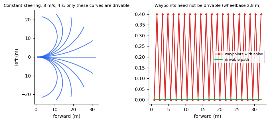
Two consequences. A trajectory's curvature is bounded by the steering limit, , so a path with sharp kinks is infeasible (curvature in the reference code
measures it from three-point circles; the test shows a 0.4 m zigzag has more than ten times the
curvature of a driven path). And the model ignores tyre slip, so it is good for ordinary driving and
wrong at the limits of grip. The NAVSIM benchmark (2406.15349)
uses an LQR controller and a kinematic bicycle model to turn a predicted trajectory into the motion
it scores.
2. The classical baseline: car following with the IDM
Before learning, a simple rule: go at your desired speed, but keep a safe gap to the car ahead. The Intelligent Driver Model (Treiber, Hennecke and Helbing, cond-mat/0002177) turns that into one formula:
Here is the desired speed, the current gap, the standstill gap, the desired time headway, the closing speed and comfortable braking. The first term accelerates on a free road; the second brakes when the gap is smaller than the wanted gap , which grows with speed and with how fast you are closing in.
def idm_acceleration(
    speed: float,
    gap: float,
    lead_speed: float,
    desired_speed: float = 15.0,
    time_headway: float = 1.5,
    min_gap: float = 2.0,
    max_accel: float = 1.5,
    comfortable_brake: float = 2.0,
) -> float:
    """Acceleration of the Intelligent Driver Model (Treiber, Hennecke and Helbing).

    The car accelerates toward ``desired_speed`` on a free road and brakes as the gap
    to the car ahead gets smaller than the gap it wants to keep, which grows with speed
    and with how fast it is closing in.

    Args:
        speed: Own speed in m/s.
        gap: Bumper-to-bumper distance to the leader in metres.
        lead_speed: Leader speed in m/s.
        desired_speed: Free-road speed.
        time_headway: Desired time gap to the leader.
        min_gap: Gap kept at standstill.
        max_accel: Maximum acceleration.
        comfortable_brake: Braking the model considers comfortable.

    Raises:
        ValueError: If ``gap`` is not positive.
    """
    if gap <= 0:
        raise ValueError(f"gap must be positive, got {gap}")
    closing = speed - lead_speed
    wanted_gap = (
        min_gap
        + speed * time_headway
        + speed * closing / (2 * math.sqrt(max_accel * comfortable_brake))
    )
    return max_accel * (1 - (speed / desired_speed) ** 4 - (wanted_gap / gap) ** 2)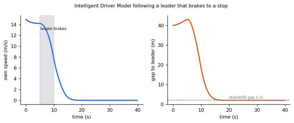
The IDM has no learning, no perception beyond the gap and speed of one leader, and it is still a strong, explainable behaviour for that one situation. It is the pattern for the rule-based half of a driving stack: a small formula with a known failure mode.
3. Rule-based planners are hard to beat in closed loop
"Parting with Misconceptions about Learning-based Vehicle Motion Planning" (2306.07962) found that simple rule-based priors, such as choosing a centerline through a lane-graph search, add value in closed-loop planning, and combined the idea into a very simple planner that won the nuPlan planning challenge 2023. It also found that the best open-loop results come from giving the model only the centerline as scene context, and that learning-based methods struggle in complex real-world scenarios. Read it as a warning about the next module: open-loop numbers and closed-loop behaviour are different things.
For a VLA researcher the lesson is practical. Always keep a rule-based baseline in your evaluation, and ask whether a learned planner beats it where it matters: rare, interactive, safety-critical cases.
4. Trajectory vocabularies
Regressing a trajectory with an L2 loss averages the possible futures (the next module shows what that does at an obstacle). One alternative is to turn planning into classification: build a large vocabulary of plausible trajectories, then score them. VADv2 (2402.13243) discretises the planning action space into a large planning vocabulary, turns the entries into planning tokens that interact with scene tokens, and outputs a probability distribution over the entries, trained from driving demonstrations.
A vocabulary is usually built by clustering logged trajectories. The reference code runs k-means on 2000 sampled drivable trajectories:
| Vocabulary size | Mean end-point error to the nearest entry |
|---|---|
| 4 | 7.09 m |
| 16 | 3.45 m |
| 64 | 1.64 m |
| 256 | 0.76 m |
Every entry in the vocabulary is drivable by construction, which answers the problem in section 1. The cost is a quantisation error that only shrinks as the vocabulary grows.
def build_vocabulary(
    trajectories: torch.Tensor, size: int, iterations: int = 30, seed: int = 0
) -> torch.Tensor:
    """K-means over flattened trajectories; the centres are the vocabulary.

    Args:
        trajectories: Shape (n, T, 2).
        size: Number of vocabulary entries.
        iterations: Lloyd iterations.
        seed: Seed for choosing the initial centres.

    Returns:
        Shape (size, T, 2).

    Raises:
        ValueError: If ``size`` is not between 1 and the number of trajectories.
    """
    if not 1 <= size <= len(trajectories):
        raise ValueError(f"size must be in [1, {len(trajectories)}], got {size}")
    flat = trajectories.flatten(1)
    generator = torch.Generator().manual_seed(seed)
    centres = flat[torch.randperm(len(flat), generator=generator)[:size]].clone()
    for _ in range(iterations):
        assignment = torch.cdist(flat, centres).argmin(dim=1)
        for k in range(size):
            members = flat[assignment == k]
            if len(members):
                centres[k] = members.mean(dim=0)
    return centres.view(size, *trajectories.shape[1:])


def quantization_error(trajectories: torch.Tensor, vocabulary: torch.Tensor) -> float:
    """Mean final-point distance from a trajectory to its nearest vocabulary entry."""
    distances = torch.cdist(trajectories.flatten(1), vocabulary.flatten(1))
    nearest = vocabulary[distances.argmin(dim=1)]
    return (trajectories[:, -1] - nearest[:, -1]).norm(dim=-1).mean().item()
Scoring can then use rules. Hydra-MDP (2406.06978) distils from both human and rule-based teachers, so the student learns how the environment shapes planning end to end, with several heads aimed at different evaluation metrics. The reference code has the simplest rule-based selector, which picks the furthest-progressing entry that does not come near an obstacle:
def select_trajectory(
    vocabulary: torch.Tensor, obstacles: torch.Tensor, radius: float = 1.5
) -> int:
    """Rule-based scoring: the furthest-progressing collision-free vocabulary entry.

    An entry collides if any of its points is within ``radius`` of an obstacle point
    (obstacles are given as (m, 2) positions). Progress is the distance of the last
    point from the origin. If every entry collides, the one that stays furthest from
    the obstacles is chosen, so the planner still returns something.

    Args:
        vocabulary: Shape (k, T, 2).
        obstacles: Shape (m, 2).
        radius: Collision distance in metres.

    Returns:
        Index of the selected entry.
    """
    flat = vocabulary.reshape(len(vocabulary), -1, 2)
    clearance = (
        torch.cdist(flat, obstacles).amin(dim=(1, 2))
        if len(obstacles)
        else (torch.full((len(vocabulary),), float("inf")))
    )
    progress = vocabulary[:, -1].norm(dim=-1)
    safe = clearance > radius
    if safe.any():
        return int(torch.where(safe, progress, torch.tensor(-1.0)).argmax())
    return int(clearance.argmax())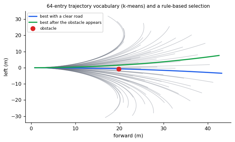
Reference implementation (PyTorch)
libs/tutorial/planning.py; tests are in libs/tutorial/tests/test_planning.py: straight driving
goes straight, constant steering draws a circle of radius , speed cannot go negative,
a zigzag has far higher curvature than a driven path, the IDM is near zero acceleration at its
desired speed, brakes when closing on a slow leader and stops behind a stopped one without touching
it, a larger vocabulary approximates better, and selection avoids an obstacle and still returns
something when everything collides. Run uv run --group tutorial python -m libs.tutorial.planning.
Check yourself
- Why is a list of waypoints not guaranteed to be drivable, and what bounds a path's curvature?
- What do the two correction terms in the IDM do?
- What does the 2023 nuPlan result say about learned versus rule-based planners?
- What do you gain and lose by planning as a choice among a vocabulary of trajectories?
Answers
- Waypoints are free positions with nothing tying them to how a car moves; noise or kinks can demand more curvature than the steering allows. The steering limit bounds curvature: |κ| ≤ tan δ_max / L.
- The (v/v₀)⁴ term cuts acceleration as the car approaches its desired speed on a free road. The (s*/s)² term brakes when the gap is smaller than the wanted gap s*, which grows with speed and with how fast the car is closing in.
- A simple planner built on a rule-based centerline prior won the 2023 nuPlan challenge, and the paper found learning-based methods struggled in complex real scenarios. Keep a rule-based baseline and ask where a learned planner beats it.
- Gain: every entry is drivable by construction, planning becomes classification (so it can pick one mode) and entries can be scored with rules. Lose: a quantisation error that shrinks only as the vocabulary grows (7.09 m at 4 entries, 0.76 m at 256), and the cost of scoring every entry.
Quiz
Answer each question; feedback appears as soon as you choose.
Sources
- Treiber, Hennecke and Helbing, Congested Traffic States in Empirical Observations and Microscopic Simulations, 2000 (introduces the IDM).
- Dauner et al., Parting with Misconceptions about Learning-based Vehicle Motion Planning, 2023.
- Jiang et al., VADv2, 2024.
- Li et al., Hydra-MDP, 2024.
- Dauner et al., NAVSIM, 2024.
Driving data and labels
Common driving datasets and benchmarks, how labels are produced and checked, and how Alpamayo-R1 builds its reasoning labels.
Predicting other drivers
Why motion prediction is multimodal, why one averaged trajectory fails, why per-agent predictions are not enough when agents interact, and how marginal and joint predictors differ.