Tokens, ViT and VLMs
How text and images become one token sequence: subword tokenizers (BPE), patch embeddings, CLIP and SigLIP, and a vision-language model built from them, with runnable code.
Text becomes tokens
A language model needs a fixed vocabulary of units. There are three obvious choices. Characters give a tiny vocabulary but very long sequences. Whole words give short sequences but an enormous vocabulary, and any unseen word breaks the model. Subwords sit between: common words are single tokens, rare words are assembled from pieces. Sennrich et al. (1508.07909) proposed splitting rare words into subword units, including pieces found by byte-pair encoding (BPE), so a translation model could handle any word with a fixed vocabulary.
Byte-pair encoding
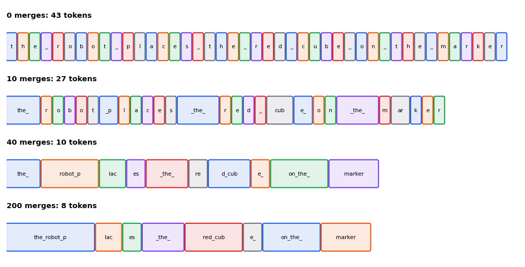
BPE learns its vocabulary from text with a very simple loop:
- Start with every byte as a token (the 256 values of UTF-8).
- Count every adjacent pair of tokens in the training text.
- Give the most frequent pair a new token id and replace every occurrence with it.
- Repeat for a chosen number of merges.
Encoding new text replays the same merges in the same order; decoding expands each token back to the bytes it stands for. Because the base alphabet is bytes, any string can be tokenized and decoded exactly, with no "unknown token". (SentencePiece, 1808.06226, is a widely used tool that learns subword units directly from raw text, with no language-specific word splitting first.)
def train_bpe(text: str, num_merges: int) -> list[tuple[int, int]]:
    """Learns merge rules from ``text``.

    Starting from the UTF-8 bytes, each step finds the most frequent adjacent pair of
    tokens and gives it a new token id. Ties are broken toward the lower ids so the
    result is deterministic.

    Args:
        text: Training text.
        num_merges: Number of merge rules to learn (the final vocabulary has
            ``256 + num_merges`` tokens, fewer if the text runs out of pairs).

    Returns:
        The merge rules in the order they were learned; rule ``i`` creates token
        ``256 + i``.
    """
    ids = list(text.encode("utf-8"))
    merges: list[tuple[int, int]] = []
    for _ in range(num_merges):
        counts = Counter(zip(ids, ids[1:], strict=False))
        if not counts:
            break
        pair = max(counts, key=lambda p: (counts[p], -p[0], -p[1]))
        ids = merge_pair(ids, pair, BASE_VOCAB + len(merges))
        merges.append(pair)
return mergesdef encode(text: str, merges: list[tuple[int, int]]) -> list[int]:
"""Tokenizes ``text`` by applying the learned merges in training order."""
ids = list(text.encode("utf-8"))
for index, pair in enumerate(merges):
ids = merge_pair(ids, pair, BASE_VOCAB + index)
return ids
def decode(ids: list[int], merges: list[tuple[int, int]]) -> str:
"""Turns token ids back into text; each token expands to the bytes it stands for."""
pieces = {i: bytes([i]) for i in range(BASE_VOCAB)}
for index, (left, right) in enumerate(merges):
pieces[BASE_VOCAB + index] = pieces[left] + pieces[right]
return b"".join(pieces[i] for i in ids).decode("utf-8", errors="replace")Tests are in libs/tutorial/tests/test_bpe.py: the first merge is the most frequent pair, encoding
then decoding returns the exact text (including emoji and random Unicode), more merges give fewer
tokens, and training stops when no pairs are left. Run uv run --group tutorial python -m libs.tutorial.bpe: 27
bytes of text became 7 tokens in our run.
Tokenization has consequences you meet later. Numbers can split into odd pieces, which is one reason writing a robot trajectory as text is awkward (the GPT-Driver entry in the Driving literature module), and why VLAs look for better action tokenizers (the Discrete tokenizers and VLA models modules). For a long, careful build-up, watch Karpathy's Let's build the GPT Tokenizer.
Embeddings and the next-token objective
Each token id indexes a row of an embedding table of shape (vocabulary, d), giving the vector the transformer works with. At the other end, a linear layer maps the last feature vector back to one score per vocabulary item (the logits), softmax makes probabilities, and training minimises the cross-entropy of the true next token (see the Transformers module). Generation repeats: predict, append, repeat. This is called autoregressive generation.
Two consequences matter for robotics:
- Anything you can turn into a token sequence can be modelled this way, including actions.
- Generation is sequential, so each new token costs a forward pass. Long outputs are slow.
Images become tokens
A Vision Transformer (ViT) (2010.11929, "An image is worth 16x16 words") treats an image like a sentence. It cuts the image into square patches, flattens each patch, projects it to a vector, adds position information, and runs a transformer over the patch sequence. There is no convolution in the backbone. With enough data it matches or beats CNNs.
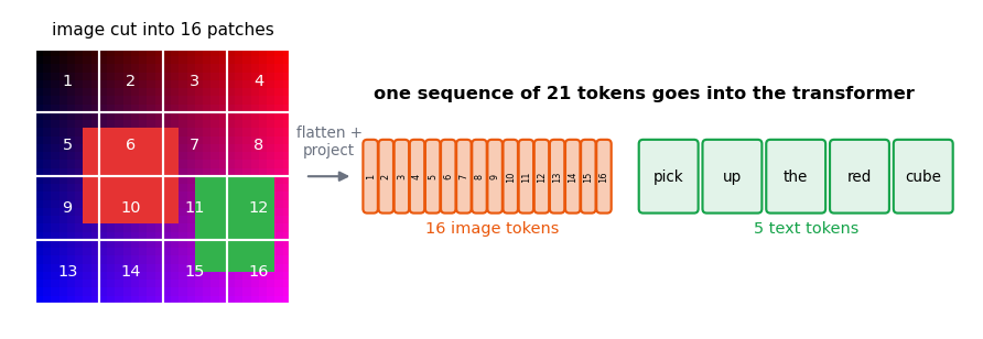
"Flatten each patch and apply one linear layer" is exactly what a convolution with kernel and stride equal to the patch size computes, which is how most implementations write it. The reference code shows both and a test checks they agree:
def patchify(images: torch.Tensor, patch_size: int) -> torch.Tensor:
    """Cuts images into flattened square patches.

    Args:
        images: Shape (batch, channels, H, W) with H and W divisible by ``patch_size``.
        patch_size: Side length of a patch in pixels.

    Returns:
        Shape (batch, num_patches, channels * patch_size * patch_size): patches in
        row-major order, each one flattened.
    """
    batch, channels, height, width = images.shape
    grid_h, grid_w = height // patch_size, width // patch_size
    patches = images.view(batch, channels, grid_h, patch_size, grid_w, patch_size)
    patches = patches.permute(0, 2, 4, 1, 3, 5)  # batch, row, column, channel, y, x
    return patches.reshape(batch, grid_h * grid_w, channels * patch_size * patch_size)
Position information for images is usually a learned vector per grid cell (our tiny ViT does that), so the model knows which patch is where.
The token budget
The number of tokens per image is , and attention cost grows with the square of the token count (the Transformers module). Halving the patch size quadruples the tokens and multiplies attention cost by about sixteen.
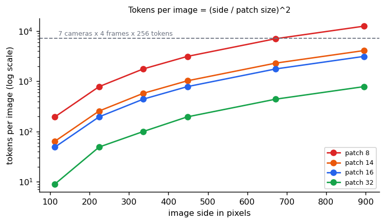
A driving car has several cameras and a history of frames, so the budget multiplies quickly. That is why SmolVLA keeps 64 visual tokens per frame and why Alpamayo-R1 studies a multi-camera tokenizer (the Sensor encoders module).
Aligning images with language: CLIP and SigLIP
CLIP (2103.00020) trains an image encoder and a text encoder together so that a matching image and caption land close together in a shared space, and mismatched pairs land far apart. Take a batch of matching pairs, normalise all the embeddings, and form the matrix of cosine similarities divided by a temperature . The diagonal holds the true pairs. A softmax cross-entropy over each row (find the right caption for each image) and over each column (find the right image for each caption), averaged, is the loss:
def clip_loss(
    image_features: torch.Tensor,
    text_features: torch.Tensor,
    temperature: float | torch.Tensor = 0.07,
) -> torch.Tensor:
    """Symmetric contrastive loss over a batch of matching image-text pairs.

    Row i of each input describes the same pair. Every other row in the batch is
    treated as a mismatch for it.

    Args:
        image_features: Shape (batch, dim).
        text_features: Shape (batch, dim).
        temperature: Divides the similarities; smaller values sharpen the softmax. It
            may be a learnable tensor, as in the CLIP paper.

    Returns:
        The mean of the image-to-text and text-to-image cross-entropy losses.
    """
    image = F.normalize(image_features, dim=-1)
    text = F.normalize(text_features, dim=-1)
    logits = image @ text.T / temperature  # (batch, batch) cosine similarities
    targets = torch.arange(len(logits))
    return (F.cross_entropy(logits, targets) + F.cross_entropy(logits.T, targets)) / 2
SigLIP (2303.15343) keeps the two encoders and changes the loss. Instead of a softmax across the batch, it scores every image-text pair on its own as a yes/no question with a sigmoid: on the diagonal and elsewhere, with a learnable scale and bias :
The paper's abstract describes the key difference: the sigmoid loss "operates solely on image-text pairs", so it does not need a global view of all pairwise similarities in the batch to normalise. The bias starts strongly negative because almost every pair in a batch is a non-match. See the paper for its results at different batch sizes.
def siglip_loss(
    image_features: torch.Tensor,
    text_features: torch.Tensor,
    log_scale: torch.Tensor,
    bias: torch.Tensor,
) -> torch.Tensor:
    """The SigLIP sigmoid loss: every image-text pair is its own yes/no question.

    Entry (i, j) of the logit matrix is scale * cos(image i, text j) + bias, and is
    pushed toward "match" on the diagonal and "no match" everywhere else. Unlike the
    softmax loss, no row or column is normalised against the others.

    Args:
        image_features: Shape (batch, dim).
        text_features: Shape (batch, dim).
        log_scale: Learnable scalar; the similarity scale is its exponential.
        bias: Learnable scalar added to every logit (it starts strongly negative,
            because almost all pairs in a batch are non-matches).

    Returns:
        The summed pairwise loss divided by the batch size.
    """
    image = F.normalize(image_features, dim=-1)
    text = F.normalize(text_features, dim=-1)
    logits = log_scale.exp() * (image @ text.T) + bias
    signs = 2 * torch.eye(len(logits)) - 1  # +1 on the diagonal, -1 elsewhere
    return -F.logsigmoid(signs * logits).sum() / len(logits)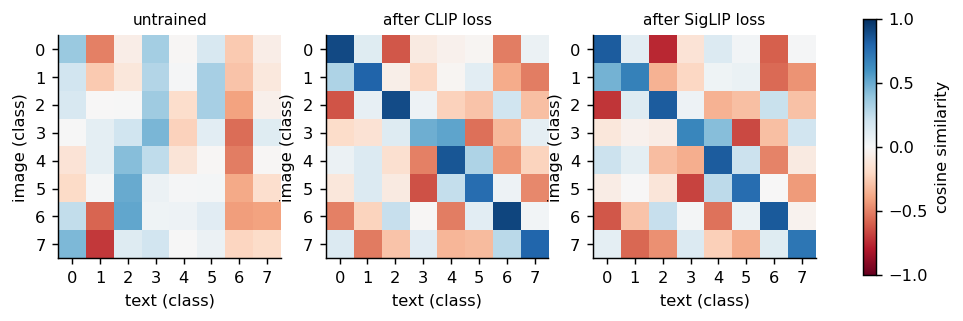
In our toy (5 seeds; uv run --group tutorial python scripts/tutorial_results.py clip_siglip), both losses learn
the scale of the similarities (CLIP's temperature starts at 0.1, SigLIP's scale at 10), and SigLIP
also learns its bias. Retrieval accuracy was 0.98 ± 0.02 with the CLIP loss and 0.99 ± 0.01 with the
SigLIP loss, against 0.12 for chance.
That difference is within noise: this toy shows that both losses learn a shared space, not that
either is better. One catch in the toy: each batch holds each class exactly once. If two items in
a batch matched, both losses would treat them as negatives, a known weakness of in-batch
negatives.
The result of either recipe is an image encoder whose features already relate to words. Many VLMs start from one: PaliGemma (2407.07726) pairs a SigLIP vision encoder with a Gemma 2B language model, and pi0 builds on PaliGemma (the VLA models module).
A vision-language model
A VLM connects a vision encoder to a language model. The common recipe: encode the image into patch tokens, project them into the language model's embedding space, and place them in the same sequence as the text tokens. The language model then reads "image tokens followed by a question" and writes text, and the whole thing is fine-tuned on image-text tasks such as captioning and question answering.
There are other ways to connect the two, each with a published example:
- Project and concatenate, as above. LLaVA (2304.08485) is described as an end-to-end trained model that connects a vision encoder and an LLM, trained on visual instruction data.
- A small learned bridge between frozen models. BLIP-2 (2301.12597) trains a lightweight Querying Transformer in two stages while the image encoder and the language model both stay frozen, which keeps training cheap.
- New layers that mix modalities inside a language model. Flamingo (2204.14198) introduces architectural innovations to bridge pretrained vision-only and language-only models and to accept interleaved images and text.
The pieces to keep in mind for the rest of the tutorial:
| Piece | Role |
|---|---|
| Vision encoder | Image to patch tokens |
| Projector | Maps vision features into the language model's input space |
| Language model | Reads the mixed sequence, writes text |
| Number of image tokens | Drives cost; fewer is faster but coarser |
A tiny VLM you can run
The toy task: a 16 by 16 image holds a red square and a green square at random positions, the question is "left", "right", "top" or "bottom", and the answer is the colour of the square in that position. Neither the image alone nor the question alone determines the answer, so the model must combine them.
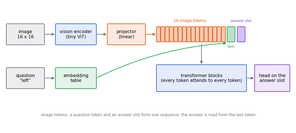
class TinyVLM(nn.Module):
    """Vision encoder, projector, and a transformer over image and text tokens."""

    def __init__(self, dim: int = 64, vision_dim: int = 48) -> None:
        """Creates the parts.

        Args:
            dim: Feature size of the language-model side.
            vision_dim: Feature size of the vision encoder's tokens.
        """
        super().__init__()
        self.vision = TinyViT(image_size=IMAGE, patch_size=4, dim=vision_dim, depth=1)
        self.projector = nn.Linear(vision_dim, dim)  # vision space -> language space
        self.question = nn.Embedding(len(QUESTIONS), dim)
        self.answer_slot = nn.Parameter(torch.zeros(1, 1, dim))
        self.blocks = nn.ModuleList(TransformerBlock(dim, heads=4) for _ in range(2))
        self.norm = nn.LayerNorm(dim)
        self.head = nn.Linear(dim, len(COLOURS))

    def forward(self, images: torch.Tensor, questions: torch.Tensor) -> torch.Tensor:
        """Returns answer logits (batch, 2) read from a learned answer token."""
        image_tokens = self.projector(self.vision(images))
        text_tokens = self.question(questions)[:, None]
        slot = self.answer_slot.expand(len(images), -1, -1)
        tokens = torch.cat([image_tokens, text_tokens, slot], dim=1)
        for block in self.blocks:
            tokens = block(tokens)
        return self.head(self.norm(tokens[:, -1]))
Tests are in libs/tutorial/tests/test_tiny_vlm.py. Run uv run --group tutorial python -m libs.tutorial.tiny_vlm
(about a minute on a laptop CPU). Over 3 seeds the accuracy was 1.00. Two checks show the answer
really depends on both inputs: shuffling the images across questions drops accuracy to 0.50 (chance
for two colours), and reversing the question (left to right, top to bottom) flips the answer in
every case. The loss sits near chance (0.69) for hundreds of steps before dropping; it first fell
below 0.4 at steps 1424, 693 and 604 for the three seeds, and in our early tries at larger
learning rates (2e-3 for 1200 steps, 1e-3 for 3000) it did not learn at all. Learning to combine two sources of information can
involve a plateau like this.
Cost
Everything in a VLM is more tokens: image tokens, text tokens and any generated reasoning. The budget above, the quadratic attention cost and the one-forward-pass-per-generated-token cost are why efficient designs compress image tokens, cache keys and values, and keep the generated part short (the Efficient fine-tuning and inference module).
A VLA is this same recipe with one more output: actions.
Reference implementation (PyTorch)
A patch embedding is a convolution whose kernel and stride equal the patch size. A tiny Vision
Transformer adds position embeddings and reuses the transformer block from the Transformers module. Tests are in
libs/tutorial/tests/test_vit.py; run the demo with uv run --group tutorial python -m libs.tutorial.vit.
class PatchEmbed(nn.Module):
    """Cuts an image into square patches and projects each to a token."""

    def __init__(
        self, image_size: int, patch_size: int, channels: int, dim: int
    ) -> None:
        """Creates the embedding.

        Args:
            image_size: Side length of the (square) input image in pixels.
            patch_size: Side length of one patch; must divide ``image_size``.
            channels: Number of image channels.
            dim: Token feature size.

        Raises:
            ValueError: If ``patch_size`` does not divide ``image_size``.
        """
        super().__init__()
        if image_size % patch_size != 0:
            raise ValueError(
                f"patch_size {patch_size} must divide image_size {image_size}"
            )
        self.num_patches = (image_size // patch_size) ** 2
        # A convolution with stride = kernel = patch size is "flatten each patch and
        # apply the same linear layer".
        self.proj = nn.Conv2d(channels, dim, kernel_size=patch_size, stride=patch_size)

    def forward(self, images: torch.Tensor) -> torch.Tensor:
        """Maps (batch, channels, H, W) to (batch, num_patches, dim)."""
return self.proj(images).flatten(2).transpose(1, 2)class TinyViT(nn.Module):
"""Patch tokens plus learned position embeddings, then transformer blocks."""
def __init__(
self,
image_size: int = 32,
patch_size: int = 8,
channels: int = 3,
dim: int = 64,
depth: int = 2,
heads: int = 4,
) -> None:
"""Creates the encoder."""
super().__init__()
self.patches = PatchEmbed(image_size, patch_size, channels, dim)
self.position = nn.Parameter(torch.zeros(1, self.patches.num_patches, dim))
nn.init.normal_(self.position, std=0.02)
self.blocks = nn.ModuleList(TransformerBlock(dim, heads) for _ in range(depth))
self.norm = nn.LayerNorm(dim)
def forward(self, images: torch.Tensor) -> torch.Tensor:
"""Maps images to one feature token per patch: (batch, num_patches, dim)."""
tokens = self.patches(images) + self.position
for block in self.blocks:
tokens = block(tokens)
return self.norm(tokens)Where to go next
- Karpathy, Let's build the GPT Tokenizer: BPE from scratch, and why tokenization causes so many model quirks.
- The ViT, CLIP and SigLIP papers linked above; the original contrastive training recipe in CLIP and the pairwise sigmoid variant in SigLIP.
- The Discrete tokenizers module for how continuous images and actions get tokens, and the VLA models module for how VLMs become robot policies.
Check yourself
- Why do subword tokenizers beat whole-word and character vocabularies for most text?
- In byte-level BPE, why can any string be encoded and decoded exactly?
- What does a ViT patch embedding compute, in terms of a linear layer?
- A CLIP batch has 8 matching pairs. What does one row of the 8 by 8 similarity matrix contain, and what is the target?
- What does SigLIP change about the CLIP loss, and what does it keep?
- In the tiny VLM, why does shuffling the images across questions drop accuracy to chance?
- How many tokens does a 336 by 336 image give with patch size 14?
- Why is writing a robot trajectory as ordinary text a poor fit for BPE tokenization?
Quiz
Answer each question; feedback appears as soon as you choose.
Sources
- Sennrich et al., Neural Machine Translation of Rare Words with Subword Units, 2015.
- Kudo and Richardson, SentencePiece, 2018.
- Dosovitskiy et al., An Image is Worth 16x16 Words, 2020 (ViT).
- Radford et al., Learning Transferable Visual Models From Natural Language Supervision, 2021 (CLIP).
- Zhai et al., Sigmoid Loss for Language Image Pre-Training, 2023 (SigLIP).
- Liu et al., Visual Instruction Tuning, 2023 (LLaVA).
- Li et al., BLIP-2, 2023.
- Alayrac et al., Flamingo, 2022.
- Beyer et al., PaliGemma, 2024.
- Van den Oord et al., Neural Discrete Representation Learning, 2017 (how continuous signals become discrete tokens).
Transformers
Self-attention, multiple heads, positions, the full block, masks and decoding, built up step by step with figures, a hand-checkable example and a tiny trained model.
Variational autoencoders
From autoencoders to VAEs: the latent-variable view, the ELBO, the closed-form KL, the reparameterisation trick, the beta trade-off and posterior collapse, with runnable code.