Efficient fine-tuning and inference
Adapting and serving large models on small hardware: LoRA and QLoRA, quantization in depth (scales, groups, outliers, int8 and 4-bit), the KV cache, FlashAttention's online softmax, speculative decoding and distillation.
Why this module
A 10-billion-parameter model has 10 billion numbers to store, differentiate and serve. At 2 bytes each (bf16) the weights alone are about 20 GB, which is why the Alpamayo-R1 weights (about 22 GB on disk) only just fit a 24 GB card (the Practices page). Full fine-tuning is worse: the Training at scale module counts 16 bytes per parameter for weights, gradients and optimiser state, about 150 GB for the same model. (The 20 GB and 150 GB figures are our arithmetic, not measurements.)
This module covers the two halves of making a large model usable on modest hardware:
- Adapting it to your task without retraining every weight: LoRA and QLoRA (sections 1 and 2).
- Running it faster and in less memory: quantization, the KV cache, FlashAttention and speculative decoding (sections 3 to 6), with distillation as the last resort (section 7).
Each technique has a toy in libs/tutorial/efficiency.py that checks the claim it rests on. For the
deadline a driving model must meet, and how these techniques fit a latency budget, continue to
Deploying a driving VLA.
1. LoRA: train a small change, not the whole model
The idea
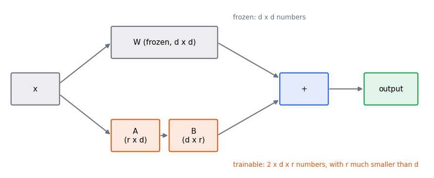
Fine-tuning changes each weight matrix by some . LoRA (2106.09685) bets that this change has low rank: that it can be written as the product of two thin matrices,
is frozen. Only and are trained: numbers instead of . For a layer and that is 131,072 instead of 16.8 million, under 1 percent. The paper reports up to 10,000 times fewer trainable parameters and 3 times less GPU memory than fully fine-tuning GPT-3 175B.
class LoRALinear(nn.Module):
    """A frozen linear layer plus a trainable low-rank update.

    The effective weight is W + (alpha / rank) * B A, where W is frozen and only the
    small matrices A (rank x in) and B (out x rank) are trained. B starts at zero, so
    the layer begins exactly equal to the pretrained one.
    """

    def __init__(self, base: nn.Linear, rank: int, alpha: float | None = None) -> None:
        """Wraps ``base``.

        Args:
            base: The pretrained layer; its parameters are frozen.
            rank: Rank of the update.
            alpha: Scale numerator; defaults to ``rank`` (a scale of 1).

        Raises:
            ValueError: If ``rank`` is not positive.
        """
        super().__init__()
        if rank < 1:
            raise ValueError(f"rank must be at least 1, got {rank}")
        self.base = base
        for parameter in self.base.parameters():
            parameter.requires_grad_(False)
        self.scale = (rank if alpha is None else alpha) / rank
        self.a = nn.Parameter(torch.randn(rank, base.in_features) / math.sqrt(rank))
        self.b = nn.Parameter(torch.zeros(base.out_features, rank))

    def forward(self, x: torch.Tensor) -> torch.Tensor:
        """Frozen output plus the low-rank correction."""
        return self.base(x) + self.scale * (x @ self.a.T @ self.b.T)

    def merge(self) -> nn.Linear:
        """Returns a plain linear layer with the update folded into the weight."""
        merged = nn.Linear(self.base.in_features, self.base.out_features)
        merged.weight.data = self.base.weight.data + self.scale * (self.b @ self.a).data
        merged.bias.data = self.base.bias.data.clone()
        return merged
Three details in the code matter in practice:
- starts at zero, so and training begins exactly at the pretrained model. A test checks the adapter's output equals the base layer's before training.
- The scale keeps the size of the update roughly independent of the rank, so a learning rate tuned at one rank still works at another.
- Merging. After training, is an ordinary matrix: fold it in and inference costs nothing extra. A test checks the merged layer gives identical outputs. (Keep the adapters separate instead if you want to swap tasks on one base model.)
What rank do you need?
If the true change has rank , an adapter of rank can represent it and a smaller one cannot. The best rank- approximation of any matrix is its truncated singular value decomposition, so we can compute the floor on LoRA's error directly:
def lora_parameters(d_in: int, d_out: int, rank: int) -> int:
    """Trainable parameters of a rank-``rank`` adapter on a d_in x d_out layer."""
    return rank * (d_in + d_out)


def best_low_rank_error(delta: torch.Tensor, rank: int) -> float:
    """Relative error of the best rank-``rank`` approximation of a weight change.

    The truncated SVD is the best possible low-rank approximation (Eckart-Young), so
    this is the floor for any LoRA adapter of that rank on that change.
    """
    u, singular, vh = torch.linalg.svd(delta, full_matrices=False)
    approx = (u[:, :rank] * singular[:rank]) @ vh[:rank]
    return ((delta - approx).norm() / delta.norm()).item()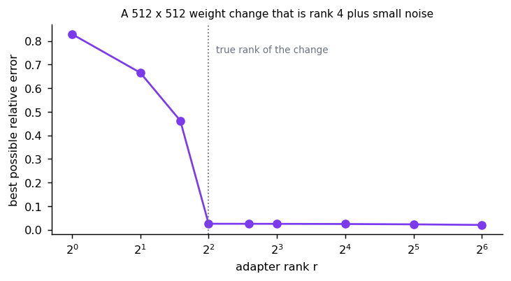
Real fine-tuning changes are not exactly low rank, but the LoRA paper's premise, borne out by its results, is that they are close to it. In practice ranks of 8 to 64 on the attention and MLP projections are common starting points; if a higher rank keeps helping on held-out data, the task is asking for more change than the adapter allows.
Where to put adapters
LoRA can wrap any linear layer. Common choices are the attention projections (query, key, value, output) and the MLP projections. For a VLA, the usual split is to adapt the language backbone and the action head and leave the vision encoder frozen, which keeps its pretrained visual features. OpenVLA's authors report fine-tuning on consumer GPUs with LoRA (the VLA models module).
2. QLoRA: fine-tune a quantized model
LoRA removes the gradients and optimiser state of the frozen weights, but the frozen weights themselves still sit in GPU memory in 16 bits. QLoRA (2305.14314) stores the frozen base model in 4 bits and backpropagates through it into 16-bit LoRA adapters. It introduces a 4-bit data type, NormalFloat (NF4), designed for normally distributed weights, and reports fine-tuning a 65B model on a single 48 GB GPU, with its Guanaco models reaching 99.3 percent of ChatGPT's performance on the Vicuna benchmark after 24 hours on one GPU.
The memory arithmetic for a 7B model, as a rough guide (our arithmetic; activations and overheads extra):
| Method | Frozen weights | Trainable state | Rough total |
|---|---|---|---|
| Full fine-tune, bf16 Adam | 16 bytes × 7B | about 104 GiB | |
| LoRA on bf16 weights | 2 bytes × 7B | small | about 13 GiB |
| QLoRA, 4-bit weights | 0.5 bytes × 7B | small | about 3.3 GiB |
That table is why QLoRA is the default way to adapt a 7B model on a 24 GB GPU.
3. Quantization: fewer bits per weight
Scale, round, clip
Quantization stores numbers in fewer bits. The simplest version, symmetric integer quantization, picks a scale so that the largest magnitude maps to the largest integer, rounds, and keeps the integers:
For 8 bits the integers run from −127 to 127; for 4 bits from −7 to 7. The rounding error per weight is at most half a step, . Inference either dequantizes to 16 bits before multiplying, which saves memory and bandwidth, or multiplies in integers directly where the hardware supports it, which also saves compute.
def quantize_int8(weight: torch.Tensor) -> tuple[torch.Tensor, torch.Tensor]:
    """Symmetric per-row int8 quantization.

    Returns:
        The int8 weights and the per-row float scale to multiply back by.
    """
    scale = weight.abs().amax(dim=1, keepdim=True).clamp(min=1e-8) / 127.0
    return (weight / scale).round().clamp(-127, 127).to(torch.int8), scale


def dequantize_int8(quantized: torch.Tensor, scale: torch.Tensor) -> torch.Tensor:
    """Maps int8 weights back to floats."""
    return quantized.float() * scale
Granularity: one scale for how many weights?
A single scale for a whole matrix (per tensor) is cheap but wasteful: one large weight stretches the scale and every small weight loses precision. Finer granularity uses more scales:
- Per row (per output channel): one scale per row.
- Per group: one scale per block of, say, 32 or 128 consecutive weights in a row. This is what most 4-bit formats do.
def quantize_dequantize(
    weight: torch.Tensor, bits: int, group_size: int | None = None
) -> torch.Tensor:
    """Symmetric integer quantization with one scale per row or per group of columns.

    Each group's scale maps its largest magnitude to the largest integer
    (2^(bits-1) - 1); values are rounded to integers and multiplied back. Smaller
    groups mean more scales to store but less damage from a single large value.

    Args:
        weight: Shape (rows, cols).
        bits: Integer width, for example 8 or 4.
        group_size: Columns per group; ``None`` uses one scale per row.

    Raises:
        ValueError: If ``group_size`` does not divide the number of columns.
    """
    rows, cols = weight.shape
    group = cols if group_size is None else group_size
    if cols % group != 0:
        raise ValueError(f"group_size {group} must divide {cols} columns")
    levels = 2 ** (bits - 1) - 1
    grouped = weight.reshape(rows, cols // group, group)
    scale = grouped.abs().amax(dim=-1, keepdim=True).clamp(min=1e-12) / levels
    return ((grouped / scale).round().clamp(-levels, levels) * scale).reshape(
        rows, cols
    )


def relative_error(weight: torch.Tensor, approx: torch.Tensor) -> float:
    """||W - W_hat|| / ||W||."""
    return ((weight - approx).norm() / weight.norm()).item()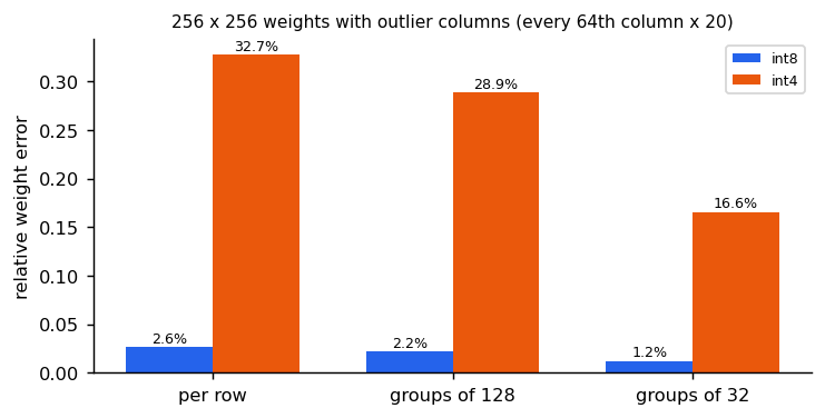
The same matrix without the outlier columns quantizes to 0.7 percent error per row at 8 bits, against 2.6 percent with them: outliers, not the bit width alone, set the error. A test checks that outliers more than double the error.
Outliers in large models
Large language models develop exactly such outliers. LLM.int8() (2208.07339) handles them with a mixed-precision decomposition: the few outlier feature dimensions are multiplied in 16 bits and more than 99.9 percent of values in 8 bits, cutting inference memory by half and running 175B-parameter models without loss. SmoothQuant and AWQ (the Deploying module) move or protect the outliers instead.
Going below 8 bits
GPTQ (2210.17323) quantizes weights to 3 or 4 bits one column at a time, adjusting the not-yet-quantized weights to compensate for each rounding error using second-order (Hessian) information from a little calibration data. It reports quantizing 175B models in about four GPU hours and speedups of about 3.25 times over fp16 on an A100 and 4.5 times on an A6000. Rule of thumb from these results: 8-bit weights are nearly free, 4-bit weights need a careful method and calibration, and below 4 bits quality drops quickly.
For a driving model, re-run the driving evaluation after quantizing, including the rare-scenario sets: an average metric can hide a loss on exactly the cases that matter (our advice; the papers above evaluate language benchmarks).
4. The KV cache
In autoregressive decoding, each new token's key and value are computed once and kept, so a new token only computes its own query, key and value instead of re-running the whole prefix. It trades memory for compute: the cache grows with layers, key-value heads, tokens and batch size, and sharing key-value heads (multi-query and grouped-query attention) shrinks it. The Transformers module has the full treatment, with a figure, the memory formula and a measured comparison. PagedAttention (2309.06180) manages the cache's memory in pages so a server can hold more sequences at once.
@torch.no_grad()
def decode_with_cache(layer: MultiHeadAttention, tokens: torch.Tensor) -> torch.Tensor:
    """Runs causal self-attention one token at a time, reusing past keys and values.

    The result equals ``layer(tokens, causal=True)`` but each new token only computes
    its own query, key and value instead of recomputing every earlier one.

    Args:
        layer: A multi-head attention layer.
        tokens: Shape (batch, n, dim).

    Returns:
        Outputs of shape (batch, n, dim).
    """
    keys: list[torch.Tensor] = []
    values: list[torch.Tensor] = []
    outputs = []
    for position in range(tokens.shape[1]):
        new = tokens[:, position : position + 1]
        keys.append(layer.split(layer.k_proj(new)))
        values.append(layer.split(layer.v_proj(new)))
        q = layer.split(layer.q_proj(new))
        k, v = torch.cat(keys, dim=2), torch.cat(values, dim=2)
        weights = (q @ k.transpose(-2, -1) / math.sqrt(q.shape[-1])).softmax(dim=-1)
        out = (weights @ v).transpose(1, 2).reshape(len(tokens), 1, -1)
        outputs.append(layer.out_proj(out))
    return torch.cat(outputs, dim=1)
5. FlashAttention: exact attention without the big matrix
Standard attention computes the full score matrix, applies the softmax and multiplies by the values. For long sequences the matrix is large, and writing it to GPU memory and reading it back costs more time than the arithmetic. FlashAttention (2205.14135) computes the same result in tiles that stay in fast on-chip memory, and never stores the full matrix. It reports a 15 percent end-to-end speedup on BERT-large, 3 times on GPT-2, and the ability to train on much longer sequences.
The trick that makes tiling possible is the online softmax. A softmax needs the maximum and the sum over the whole row, but both can be kept as running values and corrected as new blocks arrive:
and the output is at the end.
def blockwise_attention(
    q: torch.Tensor, k: torch.Tensor, v: torch.Tensor, block: int
) -> torch.Tensor:
    """Exact softmax attention computed one block of keys at a time (online softmax).

    Never forms the full (queries x keys) score matrix. For each block it keeps a
    running maximum m, a running normaliser and a running weighted sum o; when a
    later block has a larger maximum, the earlier totals are rescaled by exp(m_old -
    m_new). This is the arithmetic FlashAttention uses to keep attention inside fast
    on-chip memory.

    Args:
        q: Shape (n_q, d).
        k: Shape (n_k, d).
        v: Shape (n_k, d_v).
        block: Keys per block.
    """
    scale = q.shape[-1] ** -0.5
    m = torch.full((q.shape[0], 1), float("-inf"))
    norm = torch.zeros(q.shape[0], 1)
    o = torch.zeros(q.shape[0], v.shape[-1])
    for start in range(0, k.shape[0], block):
        scores = q @ k[start : start + block].T * scale
        m_new = torch.maximum(m, scores.amax(dim=-1, keepdim=True))
        correction = torch.exp(m - m_new)
        weights = torch.exp(scores - m_new)
        norm = norm * correction + weights.sum(dim=-1, keepdim=True)
        o = o * correction + weights @ v[start : start + block]
        m = m_new
    return o / norm
Tests check that the blockwise result equals ordinary softmax attention to for blocks of 1, 7, 16 and 64 keys. FlashAttention is exact, not an approximation: it changes where the numbers live, not what they are. That is why it is a free improvement for both training (activation memory, the Training at scale module) and inference.
6. Speculative decoding
Decoding one token at a time is limited by memory bandwidth, not arithmetic (the Deploying module): the large model reads all its weights to produce a single token. Speculative decoding (2211.17192; also 2302.01318) lets a small draft model propose tokens cheaply, then has the large target model check all in one forward pass, which costs about the same as producing one.
The verification rule keeps the output distribution exactly the target's. For each drafted token with draft probability and target probability :
- accept it with probability ;
- on rejection, sample instead from the leftover distribution , normalised, and stop.
def speculative_token(
    target: torch.Tensor, draft: torch.Tensor, generator: torch.Generator
) -> tuple[int, bool]:
    """One position of speculative sampling: the draft proposes, the target verifies.

    Draw x from the draft distribution q. Accept it with probability
    min(1, p(x) / q(x)); otherwise draw from the leftover distribution
    max(0, p - q), renormalised. The result is distributed exactly as p.

    Returns:
        The token and whether the draft's proposal was accepted.
    """
    x = int(torch.multinomial(draft, 1, generator=generator))
    accept_probability = min(1.0, (target[x] / draft[x]).item())
    if torch.rand(1, generator=generator).item() < accept_probability:
        return x, True
    leftover = (target - draft).clamp(min=0)
    token = int(torch.multinomial(leftover / leftover.sum(), 1, generator=generator))
    return token, False


def acceptance_rate(target: torch.Tensor, draft: torch.Tensor) -> float:
    """Probability that a draft token is accepted: the sum of min(p, q)."""
    return torch.minimum(target, draft).sum().item()


def expected_tokens_per_call(alpha: float, draft_length: int) -> float:
    """Expected tokens per target-model call with ``draft_length`` drafted tokens.

    The run of accepted drafts stops at the first rejection, and the target's call
    always yields one more token (the correction, or a bonus if all were accepted):
    (1 - alpha^(k+1)) / (1 - alpha) for acceptance rate alpha.
    """
    if alpha >= 1.0:
        return float(draft_length + 1)
    return (1 - alpha ** (draft_length + 1)) / (1 - alpha)


def simulate_tokens_per_call(
    target: torch.Tensor,
    draft: torch.Tensor,
    draft_length: int,
    calls: int,
    seed: int = 0,
) -> float:
    """Average tokens per target call when every position has the same p and q."""
    generator = torch.Generator().manual_seed(seed)
    produced = 0
    for _ in range(calls):
        for _ in range(draft_length):
            _, accepted = speculative_token(target, draft, generator)
            produced += 1
            if not accepted:
                break
        else:
            produced += 1  # all drafts accepted: the target call adds a bonus token
    return produced / calls
A test draws 40,000 tokens with a draft that disagrees with the target and checks the result matches the target's probabilities to within 0.01. The speed-up depends on the acceptance rate , how often the draft agrees with the target. Each target call yields tokens on average, which the reference code confirms by simulation:
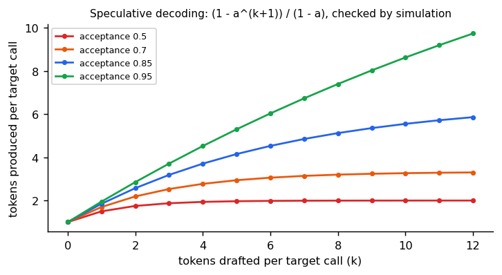
The papers report 2 to 3 times faster decoding on T5-XXL (Leviathan et al.) and 2 to 2.5 times on Chinchilla 70B (Chen et al.), with identical output distributions. For a reasoning VLA, whose reasoning tokens dominate the latency budget, this is one of the few speed-ups that cannot change behaviour.
7. Distillation
When none of the above is enough, train a smaller model to imitate the large one. Distillation has its own module, Distillation, covering soft-target knowledge distillation (1503.02531), policy and on-policy distillation, and step distillation for diffusion and flow decoders.
8. Choosing a technique
| Problem | First thing to try | Changes behaviour? |
|---|---|---|
| Adapting a large model on one GPU | LoRA; QLoRA if the base model does not fit in 16 bits | Yes (that is the point) |
| Model too large to serve | 8-bit weights; 4-bit with GPTQ or AWQ and calibration | Slightly; evaluate |
| Long sequences slow or out of memory | FlashAttention-style kernels | No (exact) |
| Decoding too slow | KV cache (always), then speculative decoding | No (exact distribution) |
| Still too slow or too large | Distil into a smaller model | Yes; evaluate on rare cases |
Reference implementation (PyTorch)
libs/tutorial/efficiency.py; tests are in libs/tutorial/tests/test_efficiency.py: the adapter
starts identical to the pretrained layer, only the two small matrices train, merging gives identical
outputs, a rank-one adapter learns a rank-one change, and a rank-4 change is captured at rank 4; int8
error stays within half a step, smaller groups and more bits reduce error, and outliers more than double
it; cached decoding equals full causal attention; blockwise attention is exact for any block size; and
speculative sampling keeps the target distribution, with the tokens-per-call formula matching
simulation. Run uv run --group tutorial python -m libs.tutorial.efficiency; in our run a rank-8 adapter on a 512 by
512 layer trains 3.0 percent of the layer's parameters.
Check yourself
- Why does LoRA initialise B to zero, and why is the update scaled by ?
- A layer gets a rank-16 adapter. What fraction of the layer's parameters is trainable?
- If a fine-tuning change has rank 4, what happens with a rank-2 adapter and with a rank-32 adapter?
- Why does QLoRA fit a 7B fine-tune on a 24 GB GPU when full fine-tuning does not?
- Why do outliers hurt per-row quantization, and how do groups help?
- How can attention be computed one block of keys at a time and still be exact?
- Why does speculative decoding not change the model's output distribution, and when does it fail to speed things up?
Answers
- B at zero makes BA zero, so training starts exactly at the pretrained model. Scaling by α / r keeps the update's size roughly independent of the rank, so a learning rate tuned at one rank still works at another.
- 16 × (4096 + 4096) = 131,072 of 16.8 million: about 0.8 percent.
- Rank 2 cannot represent a rank-4 change, so its error stays above the floor. Rank 32 can; the extra rank buys nothing beyond the noise and costs parameters.
- LoRA trains only small adapters, so there are no gradients or optimiser state for the frozen weights, and QLoRA stores those frozen weights in 4 bits: about 3.3 GiB for a 7B model instead of about 104 GiB for full fine-tuning.
- One large weight sets the scale for its whole row, so every ordinary weight in that row gets a coarse step. A group has its own scale, so outliers only coarsen the few weights in their own group.
- With the online softmax: keep a running maximum, a running sum and a running output, and rescale them as each new block of keys arrives. The final output divided by the sum equals ordinary softmax attention.
- Each drafted token is accepted with probability min(1, p / q) and a rejection resamples from the leftover of p minus q, which together reproduce the target's distribution exactly. It fails to speed things up when the draft rarely agrees with the target.
Quiz
Answer each question; feedback appears as soon as you choose.
Sources
- Hu et al., LoRA, 2021.
- Dettmers et al., QLoRA, 2023.
- Dettmers et al., LLM.int8(), 2022.
- Frantar et al., GPTQ, 2022.
- Dao et al., FlashAttention, 2022.
- Kwon et al., Efficient Memory Management for Large Language Model Serving with PagedAttention, 2023.
- Leviathan et al., Fast Inference from Transformers via Speculative Decoding, 2022.
- Chen et al., Accelerating Large Language Model Decoding with Speculative Sampling, 2023.
- Hinton et al., Distilling the Knowledge in a Neural Network, 2015.
Distillation: small, fast students from large teachers
Knowledge distillation with soft targets, feature and policy distillation, on-policy distillation, step distillation for diffusion and flow models, and how driving teams use rule-based and reasoning teachers.
Deploying a driving VLA: the onboard latency budget
Where the milliseconds go in a driving VLA and how to cut them: fewer image tokens, on-demand reasoning, fewer action steps, smaller weights, and hiding latency.