Sampling, guidance and diffusion policy
Faster samplers (DDIM and its noise knob, distillation, consistency models), the schedule mismatch that biases deterministic samplers, classifier and classifier-free guidance and what too much guidance does, and diffusion policy over action chunks, with runnable code.
The cost of sampling
Training a diffusion model is cheap (the Diffusion module), but sampling takes one network pass per step. A robot policy running at 10 Hz cannot afford hundreds of passes. This module covers three families of fixes and then the policy built on top.
Faster samplers
- DDIM (2010.02502) keeps the DDPM training procedure but uses a non-Markovian reverse process, so the same trained network can be sampled with far fewer steps; the abstract reports 10 to 50 times faster wall-clock sampling. With no added noise the sampler is deterministic. At each step it predicts the clean sample, then jumps to the next noise level:
where is the next (smaller) step in a shortened list of time steps.
- Distillation. Progressive distillation (2202.00512) trains a student to do in one step what the teacher does in two, and repeats, halving the number of steps each time.
- Consistency models (2303.01469) learn to map noise directly to data, supporting one-step generation while still allowing more steps for quality.
Flow matching (the Flow matching module) attacks the same problem from the training side by learning straighter paths.
DDIM's noise knob
DDIM is a family, not one sampler. A parameter sets how much fresh noise each jump adds:
With the sampler is deterministic: the same starting noise always gives the same sample. With it adds as much noise as the original DDPM sampler. The reference code implements the whole family:
@torch.no_grad()
def ddim_sample(
    predict_noise: NoisePredictor,
    schedule: NoiseSchedule,
    n: int,
    steps: int,
    *,
    eta: float = 0.0,
    dim: int = 2,
    start: torch.Tensor | None = None,
) -> torch.Tensor:
    """DDIM with ``steps`` jumps through the schedule; ``eta`` sets the fresh noise.

    Each jump predicts the clean sample x0 from the noise estimate, then moves to the
    next noise level. With eta = 0 the update is deterministic (DDIM); with eta = 1 it
    adds as much fresh noise as the DDPM sampler would, so eta interpolates between the
    two:

        sigma = eta * sqrt((1 - a_prev) / (1 - a_t)) * sqrt(1 - a_t / a_prev)
        x_prev = sqrt(a_prev) x0 + sqrt(1 - a_prev - sigma^2) eps + sigma z

    ``start`` replaces the usual N(0, I) starting point; use it to start from the
    true distribution of x_T when the schedule does not reach pure noise.
    """
    x = torch.randn(n, dim) if start is None else start
    times = torch.linspace(schedule.steps - 1, 0, steps).round().long()
    for i, t in enumerate(times):
        bar = schedule.alpha_bars[t]
        prev = schedule.alpha_bars[times[i + 1]] if i + 1 < steps else torch.tensor(1.0)
        eps = predict_noise(x, torch.full((n,), t.item() / schedule.steps))
        x0 = (x - (1 - bar).sqrt() * eps) / bar.sqrt()
        sigma = eta * ((1 - prev) / (1 - bar)).sqrt() * (1 - bar / prev).sqrt()
        direction = (1 - prev - sigma**2).clamp(min=0).sqrt() * eps
        x = prev.sqrt() * x0 + direction + sigma * torch.randn_like(x)
    return x
The best way to see what a sampler does is to give it a perfect noise predictor, so that every error is the sampler's own. For one-dimensional data from the optimal predictor has a closed form (the Diffusion module), and the samples should have mean 2.0 and standard deviation 0.5:
| Steps | (deterministic) | (DDPM-like) |
|---|---|---|
| 5 | mean 1.850, std 0.348 | mean 1.978, std 0.298 |
| 20 | mean 1.796, std 0.472 | mean 1.971, std 0.424 |
| 100 | mean 1.783, std 0.503 | mean 1.973, std 0.485 |
(20,000 samples; uv run --group tutorial python scripts/tutorial_results.py sampling.) Two separate effects:
- Few steps shrink the spread. With 5 jumps both samplers produce samples that are too similar (std 0.30 to 0.35 instead of 0.5). Large jumps cut the corners of the curved path, which here pulls samples towards the middle. More steps fix it.
- The deterministic sampler is biased even with 100 steps (mean 1.78 instead of 2.0), and the stochastic one is not. The reason is in the schedule, not the sampler: this toy's noise schedule ends at , not 0, so the true still contains a little signal (mean about 0.42), but sampling starts from pure . A deterministic sampler carries that starting error all the way to the end; fresh noise along the way partly washes it out. Started from the true distribution of , deterministic DDIM is exact (mean 2.00, std 0.50; a test checks it). Lin et al. (2305.08891) found the same flaw in common schedules and samplers at scale (in Stable Diffusion it limited images to medium brightness) and propose schedules that reach zero signal at the last step.
The practical lesson for a policy: test a sampler on a case where you know the answer before you trust it on one where you don't.
Guidance
Often you want to steer a conditional model: generate the path that passes above the obstacle. Classifier guidance (Diffusion Models Beat GANs, 2105.05233) needs a separate classifier. Classifier-free guidance (2207.12598) removes it: train one network on the condition and on a "no condition" token (randomly dropping the condition during training), then combine the two noise estimates at sampling time:
A larger follows the condition more strongly, usually at the cost of diversity.
Why the formula works
A noise prediction is a scaled score, the direction in which the data becomes more likely: . Classifier guidance adds the gradient of a classifier's log-probability for the condition, , scaled by : it pushes samples towards regions the classifier thinks match the condition. By Bayes' rule , which is exactly the difference between the conditional and unconditional noise estimates. Classifier-free guidance is therefore classifier guidance with an implicit classifier, the one the conditional model defines, and is how hard to push along it.
How much guidance?
@torch.no_grad()
def guidance_effect(
    model: ChunkDenoiser, schedule: NoiseSchedule, guidance: float, n: int = 1000
) -> dict[str, float]:
    """Adherence, validity and diversity of chunks asked to pass above the obstacle.

    Returns:
        ``above``: share passing above; ``clearing``: share staying outside the
        obstacle; ``spread``: standard deviation of the chunks' midpoint height among
        those passing above (a simple diversity measure).
    """
    chunks = ddim_sample(model, schedule, ABOVE, n, steps=10, guidance=guidance)
    middle = chunks[:, CHUNK // 2, 1]
    above = middle > 0
    return {
        "above": above.float().mean().item(),
        "clearing": (clearance(chunks) > OBSTACLE_RADIUS).float().mean().item(),
        "spread": middle[above].std().item() if above.sum() > 1 else 0.0,
    }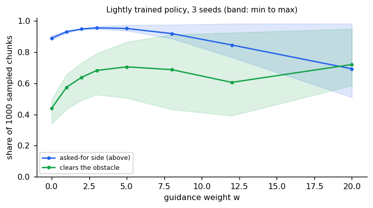
| Guidance | Passing above | Clearing the obstacle |
|---|---|---|
| 0 | 0.89 ± 0.02 | 0.44 ± 0.09 |
| 1 | 0.93 ± 0.01 | 0.57 ± 0.12 |
| 3 | 0.96 ± 0.01 | 0.68 ± 0.14 |
| 6 | 0.94 ± 0.03 | 0.71 ± 0.21 |
| 10 | 0.88 ± 0.08 | 0.66 ± 0.25 |
| 20 | 0.69 ± 0.25 | 0.72 ± 0.20 |
(3 seeds.) Moderate guidance helps both adherence and validity; past about it starts to hurt, and results swing from seed to seed. The extrapolation pushes samples beyond anything in the training data, where the network's estimates are unreliable. Even a fully trained policy, which passes above without any help, loses validity at (clearing drops from 1.00 to 0.87 in one seed; a test checks the drop). Lin et al. propose rescaling the guided prediction for the same reason. For a policy, tune on a validation set of scenes, and keep it modest.
Diffusion policy
Diffusion Policy (2303.04137) treats a visuomotor policy as a conditional denoising process over an action chunk (the Imitation learning module): condition on the observation, denoise a chunk, execute the first part, then re-plan. It handles multimodal behaviour, which a regression policy averages away. The paper benchmarks 12 tasks from 4 manipulation benchmarks and reports an average improvement of 46.9 percent over the previous state of the art; it names receding-horizon control, visual conditioning and a time-series diffusion transformer as its technical contributions.
Three horizons describe such a policy, and choosing them is most of the design:
| Horizon | What it is | Trade-off |
|---|---|---|
| Observation | How many past frames condition the model | More context versus more input to process |
| Prediction | How many future actions one denoising produces | Longer chunks are smoother and more consistent |
| Action (execution) | How many of them are executed before re-planning | Fewer means more reactive; more means fewer inference calls |
Executing only the first part of each chunk and then re-planning is receding-horizon control, the same pattern model-predictive control uses in classical driving stacks. Each re-plan costs one full sampling run, which is why the step count above and the asynchronous execution in the Deploying module matter.
Reference implementation (PyTorch)
The toy reuses the obstacle task from the imitation module. Tests are in
libs/tutorial/tests/test_diffusion_policy.py; run uv run --group tutorial python -m libs.tutorial.diffusion_policy.
class ChunkDenoiser(nn.Module):
    """Predicts the noise in a flattened action chunk, given a time and a condition."""

    def __init__(self, hidden: int = 256) -> None:
        """Creates an MLP over (noisy chunk, time, condition embedding)."""
        super().__init__()
        self.condition = nn.Embedding(3, 16)
        self.net = nn.Sequential(
            nn.Linear(CHUNK * 2 + 1 + 16, hidden),
            nn.SiLU(),
            nn.Linear(hidden, hidden),
            nn.SiLU(),
            nn.Linear(hidden, CHUNK * 2),
        )

    def forward(
        self, noisy: torch.Tensor, t_fraction: torch.Tensor, condition: torch.Tensor
    ) -> torch.Tensor:
        """Maps (batch, CHUNK * 2), (batch,), (batch,) to the predicted noise."""
        inputs = torch.cat(
            [noisy, t_fraction[:, None], self.condition(condition)], dim=-1
        )
return self.net(inputs)@torch.no_grad()
def ddim_sample(
model: ChunkDenoiser,
schedule: NoiseSchedule,
condition: int,
n: int,
steps: int = 10,
guidance: float = 0.0,
) -> torch.Tensor:
"""Samples chunks with deterministic DDIM steps and classifier-free guidance.
Args:
model: A trained denoiser.
schedule: The noise schedule it was trained with.
condition: ABOVE, BELOW or NO_CONDITION.
n: Number of chunks to sample.
steps: Number of denoising steps (a subset of the training steps).
guidance: Guidance strength w. The noise estimate becomes
(1 + w) * conditional - w * unconditional; 0 means no guidance.
Returns:
Chunks of shape (n, CHUNK, 2).
"""
x = torch.randn(n, CHUNK * 2)
times = torch.linspace(schedule.steps - 1, 0, steps).long()
cond = torch.full((n,), condition)
uncond = torch.full((n,), NO_CONDITION)
for i, t in enumerate(times):
t_fraction = torch.full((n,), t.item() / schedule.steps)
eps = model(x, t_fraction, cond)
if guidance > 0.0:
eps = (1 + guidance) * eps - guidance * model(x, t_fraction, uncond)
bar = schedule.alpha_bars[t]
previous = (
schedule.alpha_bars[times[i + 1]] if i + 1 < steps else torch.tensor(1.0)
)
x0 = (x - (1 - bar).sqrt() * eps) / bar.sqrt()
x = previous.sqrt() * x0 + (1 - previous).sqrt() * eps
return x.view(n, CHUNK, 2)What we measured: 1000 chunks per setting, mean and standard deviation over 3 training seeds
("clearing" means the path stays outside the obstacle). uv run --group tutorial python scripts/tutorial_results.py diffusion_policy reproduces the table.
| Setting | Clearing the obstacle | Passing above |
|---|---|---|
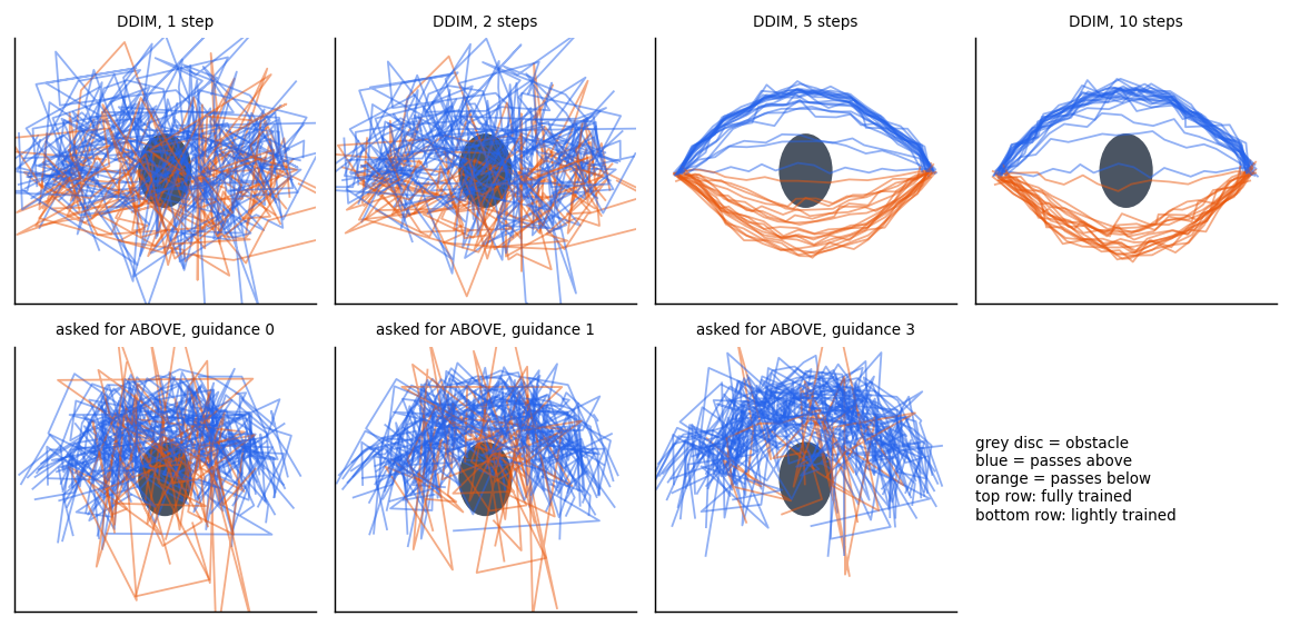
| Fully trained, no condition, 1 DDIM step | 0.35 ± 0.01 | 0.49 ± 0.07 |
| Fully trained, no condition, 2 steps | 0.35 ± 0.02 | 0.48 ± 0.07 |
| Fully trained, no condition, 5 steps | 0.80 ± 0.03 | 0.50 ± 0.02 |
| Fully trained, no condition, 10 steps | 0.86 ± 0.02 | 0.51 ± 0.02 |
| Fully trained, no condition, 50 steps | 0.90 ± 0.03 | 0.51 ± 0.01 |
| Lightly trained, asked for above, guidance 0 | 0.44 ± 0.09 | 0.89 ± 0.02 |
| Lightly trained, asked for above, guidance 1 | 0.57 ± 0.12 | 0.93 ± 0.01 |
| Lightly trained, asked for above, guidance 3 | 0.68 ± 0.14 | 0.96 ± 0.01 |
Reading the table: one or two steps give mostly invalid paths, five already works, and about ten is close to the 50-step result, as with flow matching. The figure above shows one training seed. Guidance helps most when the conditional model is imperfect. A fully trained model already follows the condition, so guidance adds little there.
Check yourself
- What does DDIM change: the training procedure or the sampling procedure?
- Why must the condition be randomly dropped during training for classifier-free guidance?
- What is the cost of a very large guidance weight?
- Why is a diffusion policy better than a regression policy when two paths are equally good?
- What does DDIM's control, and why was the deterministic sampler biased in the toy while the stochastic one was not?
- Why is classifier-free guidance a form of classifier guidance, and what goes wrong when is very large?
- What do the observation, prediction and action horizons of a diffusion policy trade off?
Quiz
Answer each question; feedback appears as soon as you choose.
Sources
- Song et al., Denoising Diffusion Implicit Models, 2020.
- Salimans and Ho, Progressive Distillation for Fast Sampling of Diffusion Models, 2022.
- Song et al., Consistency Models, 2023.
- Dhariwal and Nichol, Diffusion Models Beat GANs on Image Synthesis, 2021.
- Ho and Salimans, Classifier-Free Diffusion Guidance, 2022.
- Chi et al., Diffusion Policy, 2023.
- Lin et al., Common Diffusion Noise Schedules and Sample Steps are Flawed, 2023.
Flow matching
Learning a velocity field that carries noise to data: the objective, what the network really learns, why paths curve and how reflow straightens them, ODE solvers, conditioning for robot policies, and how it relates to diffusion.
Imitation learning and action chunking
Behaviour cloning, why it drifts (measured on a lane-keeping toy), DART and DAgger, action chunks and temporal ensembling, and why generative policies help, with our SO-100 measurements.