Sensor encoders for driving
How cameras, lidar, radar, maps and vehicle state become tokens or feature maps: lifting camera features along rays into a bird's-eye view, pillar and polyline encoders, a fusion experiment, calibration and time synchronisation, and the compute each choice costs.
Sources and confidence
Paper claims come from the arXiv abstracts. General statements (for example how radar works) are standard background and are not tied to one paper. The exercise was run.
The common problem
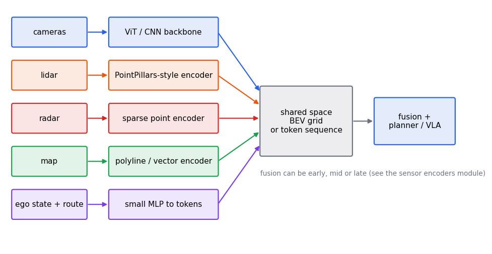
A driving model receives very different signals: images, 3D point clouds, sparse radar returns, a map, and the car's own motion. Each has a different shape and geometry. Every system needs (1) an encoder per modality that turns raw data into features, and (2) a shared representation where those features meet. Two shared representations dominate:
- Bird's-eye view (BEV): a top-down grid of features around the car. Good for planning because distances and free space are explicit.
- A token sequence: every modality becomes tokens in one transformer (the Transformers module), which then attends across all of them.
Cameras
Per-camera features come from a CNN or ViT backbone (the Tokens, ViT and VLMs module). The hard part is going from 2D images to the 3D world.
- Lift-Splat-Shoot (2008.05711) "lifts" each image into a frustum of features and "splats" all cameras' frustums onto a BEV grid, learning to fuse the whole camera rig.
- BEVFormer (2203.17270) uses a grid of BEV queries that pull features from the cameras by spatial cross-attention, and a temporal self-attention over past BEV maps, so history is fused too.
- PETR (2203.05625) skips BEV: it encodes 3D coordinates into the image features, so object queries can reason in 3D directly.
Lift-splat, step by step
Lift-Splat-Shoot's core is small enough to run. A forward camera has image columns, each looking along a bearing. For each column the network predicts a feature vector and a probability over a set of candidate depths. The two steps:
- Lift. Multiply the feature by each depth's probability, producing one weighted copy of the feature at each candidate point along the column's ray (an outer product: features × depths).
- Splat. Add every lifted feature into the BEV cell its 3D point falls in. Many rays and depths land in the same cell, and their contributions add.
def lift_splat(
    features: torch.Tensor,
    depth_probs: torch.Tensor,
    depths: torch.Tensor,
    angles: torch.Tensor,
    grid: int = 32,
    cell: float = 1.0,
) -> torch.Tensor:
    """Lifts per-column camera features into a BEV grid, spreading them along each ray.

    A forward camera has ``W`` image columns, each looking along a bearing angle. For
    column w, the network predicts a feature vector (C) and a probability over ``D``
    candidate depths. The **lift** step forms the outer product: the feature, weighted
    by each depth's probability, at each of the D points along the ray. The **splat**
    step adds every lifted feature into the BEV cell that point falls in.

    Args:
        features: Shape (W, C).
        depth_probs: Shape (W, D), rows sum to 1.
        depths: Candidate depths in metres, shape (D,).
        angles: Bearing of each column in radians (0 is straight ahead), shape (W,).
        grid: BEV cells per side; x (forward) spans [0, grid * cell); y is centred.
        cell: Cell size in metres.

    Returns:
        BEV features of shape (C, grid, grid), indexed [channel, x cell, y cell].
    """
    c = features.shape[1]
    lifted = features[:, None, :] * depth_probs[:, :, None]  # (W, D, C)
    x = depths[None, :] * torch.cos(angles)[:, None]  # (W, D) forward distance
    y = depths[None, :] * torch.sin(angles)[:, None]  # (W, D) lateral offset
    ix = (x / cell).floor().long()
    iy = (y / cell + grid / 2).floor().long()
    inside = (ix >= 0) & (ix < grid) & (iy >= 0) & (iy < grid)
    flat = (ix * grid + iy)[inside]
    bev = torch.zeros(grid * grid, c)
    bev.index_add_(0, flat, lifted[inside])
    return bev.view(grid, grid, c).permute(2, 0, 1).contiguous()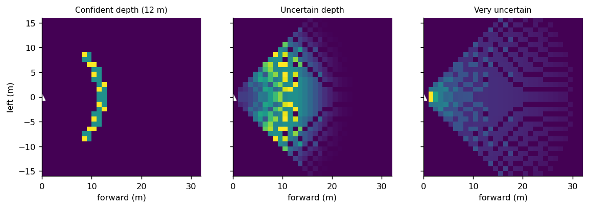
Tests check the geometry: a confident depth lands the feature in the cell on the ray, an off-axis ray lands to the side, an uncertain depth smears the feature across the cells along the ray while its total is preserved, and points outside the grid are dropped. Two consequences matter in practice:
- Depth is the hard part. A pixel is a ray (Camera geometry and object queries); the depth distribution says where on it the object is. A wrong depth puts a car in the wrong cell, so depth supervision (from lidar) and accurate camera calibration decide the quality of the BEV.
- BEVFormer removes the explicit depth. Its BEV queries project their own 3D positions into each camera and attend to the features around the projected point (the reverse direction), so depth is resolved by attention rather than by an explicit distribution.
Token cost. Tokens per input = cameras x frames x patches per image. As an illustration (not any particular system), 7 cameras x 4 frames x 256 patches is 7,168 tokens, before any text. That is why VLM-based driving models compress image tokens, as SmolVLA does for robot arms (the VLA models module).
The Alpamayo-R1 paper reports the same problem. It notes that standard VLMs process frames independently, giving token counts too large for real-time inference with many cameras, and studies a multi-camera tokenizer that needs 288 tokens per timestep however many cameras there are (about 41 tokens per image for a 7-camera vehicle, 3.9 times fewer than single-image tokenization). Its default tokenizer, used for its experiments, is still the VLM's own vision encoder applied to each image.
Lidar
A lidar scan is an unordered set of 3D points, which a CNN cannot read directly. Three approaches:
- Points: PointNet (1612.00593) consumes the raw set with a shared per-point network and a symmetric pooling, so point order does not matter.
- Voxels: VoxelNet (1711.06396) groups points into 3D cells and learns a feature for each.
- Pillars: PointPillars (1812.05784) groups points into vertical columns, runs a PointNet in each, and scatters the result into a BEV image so a normal 2D CNN can finish the job. Its paper reports it is faster than earlier encoders.
CenterPoint (2006.11275) then detects and tracks objects as points on the BEV map.
Exercise: a pillar encoder in NumPy
Random points are grouped into 0.5 m pillars over an 80 m square, passed through a shared linear layer, and max-pooled per pillar into a BEV feature map. We ran it:
import numpy as np

rng = np.random.default_rng(0)
points = np.column_stack(
    [rng.uniform(-40, 40, 20000), rng.uniform(-40, 40, 20000),
     rng.uniform(-2, 2, 20000), rng.uniform(0, 1, 20000)]
)  # x, y, z in metres, intensity

CELL = 0.5
SIZE = 160  # 160 cells of 0.5 m = 80 m
ix = ((points[:, 0] + 40) / CELL).astype(int)
iy = ((points[:, 1] + 40) / CELL).astype(int)
pillar = ix * SIZE + iy

W = rng.standard_normal((4, 16))
features = np.maximum(points @ W, 0)  # shared per-point linear layer + ReLU

bev = np.zeros((SIZE * SIZE, 16))
np.maximum.at(bev, pillar, features)  # max-pool the points in each pillar
bev = bev.reshape(SIZE, SIZE, 16).transpose(2, 0, 1)

occupied = len(np.unique(pillar))
print("BEV feature map shape (C, H, W):", bev.shape)
print("occupied pillars:", occupied, "of", SIZE * SIZE)

shuffled = rng.permutation(len(points))
bev2 = np.zeros_like(bev.reshape(16, -1).T)
np.maximum.at(bev2, pillar[shuffled], features[shuffled])
print("point order does not matter:", np.allclose(bev2.T.reshape(16, SIZE, SIZE), bev))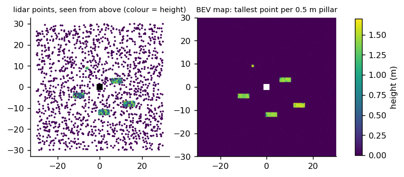
The same encoder in PyTorch, with the scatter done by a max-reduction instead of a loop:
def pillar_encode(
    points: torch.Tensor,
    weight: torch.Tensor,
    size: int = 160,
    cell: float = 0.5,
    half_range: float = 40.0,
) -> torch.Tensor:
    """PointPillars-style encoding: shared per-point layer, then max-pool per pillar.

    Args:
        points: Shape (N, F) with columns x, y first (metres) and any other features.
        weight: Shared linear layer, shape (F, K).
        size: Grid cells per side.
        cell: Cell size in metres.
        half_range: The grid covers [-half_range, half_range) in x and y.

    Returns:
        BEV feature map of shape (K, size, size). Empty pillars are zero.
    """
    ix = ((points[:, 0] + half_range) / cell).long().clamp(0, size - 1)
    iy = ((points[:, 1] + half_range) / cell).long().clamp(0, size - 1)
    features = torch.relu(points @ weight)
    bev = torch.zeros(size * size, weight.shape[1])
    index = (ix * size + iy)[:, None].expand_as(features)
    bev.scatter_reduce_(0, index, features, reduce="amax", include_self=True)
    return bev.view(size, size, -1).permute(2, 0, 1).contiguous()
A test checks that shuffling the points gives the same map (up to float rounding) and that a point's cell holds at least that point's own feature (max-pooling can only raise it).
Output of the NumPy version: shape (16, 160, 160), 13895 of 25600 pillars occupied, and True for
order invariance. The occupancy is high only because the points are uniform random; a real scan is
denser near the car and empty in many cells. The point to take away: a max-pool over a set makes
the encoder independent of point order, and the output is an image a CNN or ViT can read.
What lidar costs
The BEV grid sets the compute. At 0.5 m cells over 80 m the map has pillars; at 0.25 m it has 102,400, four times as many cells for each CNN layer, though a real scan fills only a fraction. The trade-offs: smaller cells keep small objects (pedestrians, cyclists) but cost compute and need denser points to be meaningful; larger ones are cheap and blur. A reasonable design question to ask of any lidar paper is the cell size, the range and the number of points per pillar it keeps.
Radar
Radar returns are far sparser and noisier than lidar, but they measure range precisely at long distance, can measure radial velocity directly (Doppler), and work in rain, fog and darkness. CRN (2304.00670) uses sparse but accurate radar points to help lift camera features into BEV, then fuses image and radar BEV features with deformable attention that tolerates misalignment between the two. Its paper reports real-time operation at 20 FPS.
Fusion
Why fuse at all: an experiment
Each sensor measures a different thing, and a decision can need both. In the toy, an object is a car or a pedestrian (the camera sees which, but not where) at a lateral offset (lidar measures where, but cannot tell which). The right action, "brake", applies only to a car in our lane. A small network is trained on one sensor or on both (concatenated features), with noise in each:
def fusion_scenes(
    n: int, seed: int = 0, camera_noise: float = 0.5, lidar_noise: float = 0.15
) -> tuple[torch.Tensor, torch.Tensor, torch.Tensor]:
    """Scenes where the right decision needs both sensors.

    An object is a car or a pedestrian (the camera sees which, but not where) at a
    lateral offset (lidar measures where, but cannot tell which).
    The decision "brake" is right only for a car that is in our lane.

    Returns:
        Camera features (n, 4), lidar features (n, 4), labels (n,).
    """
    generator = torch.Generator().manual_seed(seed)
    is_car = torch.rand(n, generator=generator) < 0.5
    offset = (torch.rand(n, generator=generator) - 0.5) * 6.0
    label = is_car & (offset.abs() < 1.5)
    appearance = torch.stack([is_car.float(), 1.0 - is_car.float()], dim=-1)
    camera = torch.cat(
        [
            appearance + camera_noise * torch.randn(n, 2, generator=generator),
            torch.randn(n, 2, generator=generator),  # texture: no information
        ],
        dim=-1,
    )
    lidar = torch.cat(
        [
            offset[:, None] + lidar_noise * torch.randn(n, 1, generator=generator),
            torch.randn(
                n, 3, generator=generator
            ),  # height, intensity, range: no information
        ],
        dim=-1,
    )
    return camera, lidar, label.long()


def train_fusion(mode: str, steps: int = 1200, seed: int = 0) -> float:
    """Trains a small MLP on one sensor or both and returns test accuracy.

    Args:
        mode: ``"camera"``, ``"lidar"`` or ``"both"`` (concatenated features).

    Raises:
        ValueError: If ``mode`` is unknown.
    """
    if mode not in ("camera", "lidar", "both"):
        raise ValueError(f"mode must be camera, lidar or both, got {mode!r}")
    cam, lid, y = fusion_scenes(3000, seed)
    test_cam, test_lid, test_y = fusion_scenes(5000, seed + 100)

    def pick(camera: torch.Tensor, lidar: torch.Tensor) -> torch.Tensor:
        both = torch.cat([camera, lidar], dim=-1)
        return {"camera": camera, "lidar": lidar, "both": both}[mode]

    x, test_x = pick(cam, lid), pick(test_cam, test_lid)
    torch.manual_seed(seed)
    net = nn.Sequential(nn.Linear(x.shape[1], 32), nn.ReLU(), nn.Linear(32, 2))
    optimizer = torch.optim.Adam(net.parameters(), lr=1e-2)
    for _ in range(steps):
        loss = nn.functional.cross_entropy(net(x), y)
        optimizer.zero_grad()
        loss.backward()
        optimizer.step()
    with torch.no_grad():
        return (net(test_x).argmax(dim=1) == test_y).float().mean().item()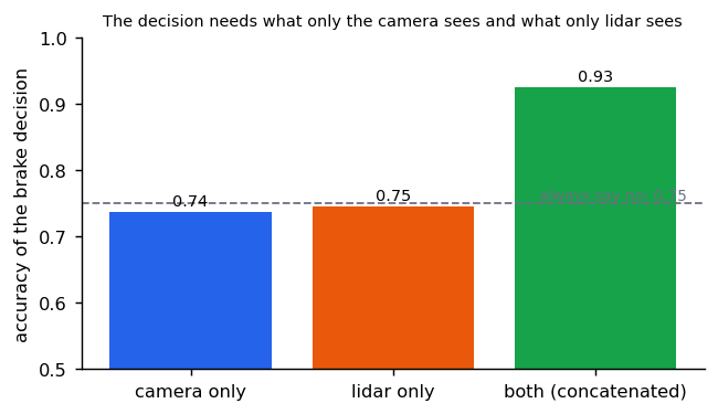
Neither sensor alone does better than the 0.75 you get by always saying no, because each is missing half of what the decision needs; together they reach 0.92 to 0.93. Real sensors overlap more than this, but the principle holds: fusion is worth the most where the sensors' failures differ (a camera at night, lidar in heavy rain, radar on a stationary object).
Where to fuse
How do the modality features meet?
| Pattern | How | Example |
|---|---|---|
| Point-level | Paint camera features onto lidar points | Older fusion; the BEVFusion paper argues it throws away camera semantic density |
| BEV-level | Each modality to BEV, then concatenate or attend | BEVFusion (2205.13542): camera and lidar in a shared BEV space, task-agnostic |
| Transformer-level | Attention across modality features | TransFuser (2205.15997): self-attention fuses perspective-view image and BEV lidar features at several resolutions; the paper reports 48% fewer collisions per kilometre than geometry-based fusion in CARLA |
| Token-level | All modalities as tokens in one sequence | Wayformer (2207.05844) compares early, late and hierarchical fusion for motion forecasting |
Practical problems that fusion papers gloss over
- Calibration. Every projection above assumes known extrinsics and intrinsics. A camera that has shifted by half a degree moves a car 10 m away by about 9 cm and one 100 m away by about 87 cm (arc length is distance times angle: rad), so long-range objects suffer most. Fusion methods that tolerate misalignment (CRN's deformable attention, mentioned above) exist for this reason.
- Time synchronisation. Sensors sample at different instants: a lidar sweep takes 100 ms, a camera exposes in milliseconds, and a vehicle at 20 m/s moves 2 m in 100 ms. Points are usually motion-compensated to a common timestamp with the ego-motion transform from Camera geometry and object queries; features from different times need the same treatment.
- Missing sensors. A camera can be blocked and a lidar can fail. Systems that were only ever trained with every sensor present can fail badly when one drops out; training with random modality dropout is the common remedy (our general recommendation, not a claim from one paper).
Beyond a flat BEV: occupancy and scene reconstruction
A bird's-eye-view map keeps one value per ground cell (for example the tallest point), so anything stacked vertically is collapsed. 3D occupancy keeps a grid of voxels and says which are occupied, so overhangs, gantries and tree branches survive.
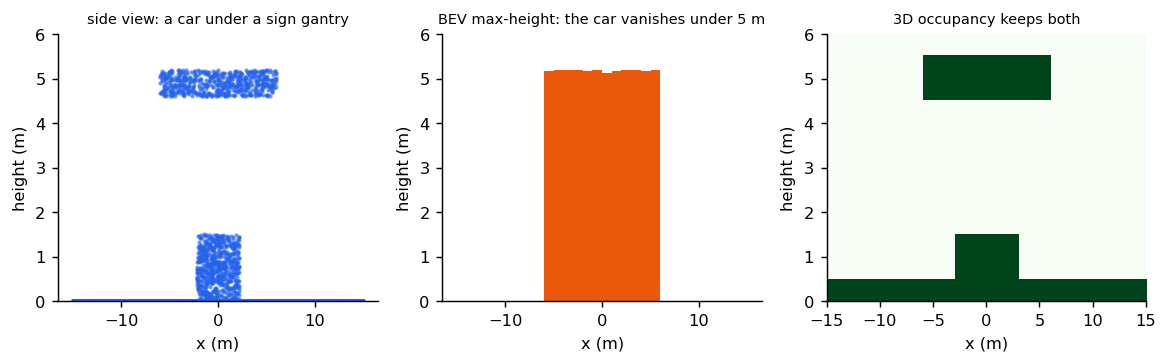
- TPVFormer (2302.07817) uses a tri-perspective view to predict 3D semantic occupancy from images.
- Occ3D (2304.14365) provides occupancy benchmarks built on Waymo and nuScenes, with a label pipeline of voxel densification, occlusion reasoning and image-guided refinement.
Neural scene reconstruction. NeRF (2003.08934) represents a scene as a network from a 5D coordinate (position and viewing direction) to density and colour, rendered by volume rendering. 3D Gaussian Splatting (2308.04079) represents it as many 3D Gaussians for real-time rendering. Street Gaussians (2401.01339) model dynamic urban scenes from video, with separate foreground vehicles and background, enabling editing and fast rendering. Our reading of why this matters for driving: a reconstructed logged drive can be re-rendered and edited, which is a route to more realistic closed-loop test scenes than hand-built ones.
The map as a sensor
A high-definition (HD) map gives lane geometry, boundaries, crosswalks and traffic-light state. Two choices:
- Render it as an image and use a CNN. Simple, but rendering loses precision.
- Keep it vectorised. VectorNet (2005.04259) encodes each lane or agent trajectory as a polyline of vectors, runs a graph network over each polyline, then models interactions among all of them, avoiding lossy rendering.
class PolylineEncoder(nn.Module):
    """VectorNet's polyline subgraph: encode vectors, pool, repeat.

    A lane is a sequence of points. Each segment becomes a vector (start, end, and its
    own attributes). Using differences between points rather than absolute coordinates
    makes the encoding independent of where the lane is in the world.
    """

    def __init__(self, dim: int = 32) -> None:
        """Creates one message-passing layer: a shared MLP and a pooled summary."""
        super().__init__()
        self.first = nn.Sequential(nn.Linear(4, dim), nn.ReLU())
        self.second = nn.Sequential(nn.Linear(2 * dim, dim), nn.ReLU())

    def forward(self, points: torch.Tensor) -> torch.Tensor:
        """Encodes one polyline of shape (n_points, 2) into a vector (dim,)."""
        start, end = points[:-1], points[1:]
        vectors = torch.cat([end - start, start - start[0]], dim=-1)  # relative only
        hidden = self.first(vectors)
        pooled = hidden.max(dim=0).values
        mixed = torch.cat([hidden, pooled.expand_as(hidden)], dim=-1)
        return self.second(mixed).max(dim=0).values
The code makes VectorNet's key design choice explicit: each segment is described by the vector between its endpoints and its offset from the polyline's start, never by absolute coordinates. A test shifts a lane by (100, −50) metres and gets the same encoding, while bending the lane changes it. That is what lets one network read lanes anywhere in the world, and why vectorised maps scale better than rendering them as images at a fixed position.
HD maps are costly to build and keep current, so many systems predict the map online from sensors. MapTR (2208.14437) builds a vectorised HD map from camera input with a transformer, modelling each element as a set of points; its paper reports a real-time variant at 25.1 FPS on an RTX 3090.
Ego state and history
The car's own speed, acceleration, steering and recent poses are small vectors. The usual encoding: a small MLP or a linear layer projects each time step to a token or a feature, with position information added so the model knows the order. The routing intent (turn left, go straight) is added the same way. Alpamayo-R1 uses the vehicle's recent motion as an input alongside multi-camera video, and the open repository says route and navigation conditioning was not released (see Driving VLA concepts).
What each choice costs
Rough orders of magnitude help decide where a sensor belongs (our arithmetic for illustrative setups, not measurements of any system):
| Input | Typical size | Tokens or cells | Note |
|---|---|---|---|
| 7 cameras × 4 frames × 256 patches | 28 images | 7,168 tokens | Attention cost grows with the square of this |
| The same, compressed to 41 tokens per image (Alpamayo-R1's multi-camera tokenizer, 288 per timestep) | 288 tokens per timestep | 3.9× fewer than per-image tokens | |
| Lidar BEV, 80 m at 0.5 m | 25,600 pillars | CNN cost scales with cells, not points | |
| Vectorised map, 100 lanes × 20 points | 100 polylines | Cheap; independent of range | |
| Ego state, 10 past poses | 10 tokens or one vector | Negligible |
The lesson: cameras dominate tokens, lidar dominates grid cells, and the map and ego state are almost free. Compression of the camera stream is where onboard budgets are won or lost (Deploying a driving VLA).
Where VLA driving models sit
Classic perception stacks (BEVFusion, TransFuser) fuse many sensors into one BEV and then plan. Many recent driving VLAs (the Driving literature module) feed cameras and ego motion directly into a VLM and output a trajectory, trading explicit multi-sensor geometry for scale and language reasoning. Whether a VLA should also take lidar, radar and maps is an open design question; treat any claim that one choice is best with caution unless it is tested closed loop on the same benchmark.
Reference implementation (PyTorch)
libs/tutorial/sensor_encoders.py; tests are in libs/tutorial/tests/test_sensor_encoders.py:
lift-splat puts a confident feature in the right cell, an off-axis ray to the side, smears an uncertain
depth while preserving its total and drops points outside the grid; pillars ignore point order;
polyline encodings ignore translation but not shape; two sensors beat either alone on the toy; and the
token-budget and bearing helpers. There is no demo script: the tests are the demonstration.
Check yourself
- Why can a CNN not read a lidar point cloud directly, and how does PointPillars get around it?
- What property of max-pooling makes a point-set encoder independent of point order?
- Name one reason to use radar when a camera and lidar are already present.
- What do you lose by rendering an HD map to an image, and how does VectorNet avoid it?
- Compute the token count for 6 cameras, 2 frames and 196 patches per image.
- In lift-splat, what does the depth distribution do, and what happens to the BEV when it is wrong?
- Why do relative vectors make a map encoder independent of where the lane is?
- A camera drifts by 0.5° in yaw. How far does that move an object at 50 m?
- Why can two sensors beat either alone, and where would you expect fusion to help most?
Answers
- A CNN expects a dense, regular grid; a point cloud is an unordered, sparse set whose size changes from scan to scan. PointPillars groups points into vertical columns over a BEV grid, encodes each column's points with a shared per-point layer and max-pooling, and scatters the column features into a 2D image that an ordinary CNN can read.
- Max is symmetric: it gives the same answer whatever order its inputs come in. Because the same per-point layer is applied to every point, shuffling the points only shuffles the inputs to the max, so the output does not change.
- Radar measures radial velocity directly (Doppler), measures range accurately at long distance, and keeps working in rain, fog and darkness, where cameras and lidar degrade.
- Rendering fixes a resolution and a position, so fine geometry is lost and range is capped by the image size. VectorNet keeps each lane or trajectory as a polyline of vectors, encodes each polyline with a graph network and then models interactions among polylines.
- 6 cameras × 2 frames × 196 patches = 2,352 tokens, before any text.
- It decides where along each pixel's ray the feature is placed: each candidate depth receives a copy weighted by its probability. A wrong depth puts the feature, say a car, in the wrong BEV cell; an uncertain one smears it along the ray.
- Each segment is described by the vector between its endpoints and its offset from the start of the polyline, never by absolute coordinates. Moving the whole lane leaves every relative vector unchanged; the test shifts a lane by (100, −50) m and gets the same encoding.
- Arc length is distance times angle: 50 m × 0.0087 rad ≈ 0.44 m.
- Each sensor measures part of what the decision needs: in the toy the camera knows what the object is and lidar knows where it is. Alone each scored 0.74, below the 0.75 of always answering no; together they reached 0.93. Fusion helps most where the sensors fail differently: cameras at night, lidar in heavy rain, radar on stationary objects.
Quiz
Answer each question; feedback appears as soon as you choose.
Sources
Every paper above is linked inline; titles and identifiers were checked on arXiv.
From modular stacks to end-to-end driving
For engineers who built perception, prediction and planning modules: what end-to-end learning replaces, what it keeps, where hand-designed interfaces lose information, and how hybrid stacks combine both.
Camera geometry and object queries
Coordinate frames, intrinsics and extrinsics, ego-motion compensation, and how DETR-style queries and Hungarian matching turn a set of objects into a loss.