Before you start
What the tutorial assumes, with a refresher on each piece: tensors and shapes, MLPs, losses and stable cross-entropy, backpropagation by hand, optimisers, overfitting and regularisation, embeddings, and entropy, cross-entropy and KL divergence.
Who this page is for
The tutorial assumes you can train a small neural network: you know what a loss, a gradient and a mini-batch are, and you have seen an MLP and a CNN. This page lists what is assumed and then refreshes each piece at the depth the later modules rely on, with code you can run. If everything here is familiar, take the self-test at the end and go straight to Transformers. If a section is new, it is worth an hour before continuing: every later module uses it.
You should already know
- How a neural network is trained: a loss, backpropagation, gradient descent and mini-batches.
- What an MLP, a convolution layer and a CNN are.
- What softmax and cross-entropy do, and what an embedding is.
- Basic probability: a distribution, a mean, a standard deviation, a Gaussian.
- Enough Python and PyTorch (or NumPy) to read a short script.
For the robotics and driving modules, it helps to know what a joint, a trajectory and a controller are.
What you do not need
Transformers, VAEs, diffusion, flow matching, reinforcement learning and world models are taught from scratch. Engineers coming from modular autonomous-driving stacks may want to read From modular stacks to end-to-end early.
1. Tensors and shapes
Almost every bug in model code is a shape bug, so the tutorial writes shapes in comments and
docstrings, such as (batch, n, dim). The conventions used throughout:
| Symbol | Meaning | Example |
|---|---|---|
| batch | Independent examples processed together | 64 images |
| n, seq | Positions in a sequence (tokens, time steps) | 196 image patches |
| dim, d | Features per position | 768 |
| heads | Attention heads | 12 |
A linear layer maps the last dimension and leaves the others alone: (batch, n, 768) → (batch, n, 3072). Matrix multiplication with @ works on the last two dimensions and broadcasts over the
leading ones, which is why the same code handles one example or a whole batch.
2. An MLP, forward
A multilayer perceptron alternates linear maps and nonlinearities:
Without the nonlinearity, two linear layers collapse into one ( is still linear), so the activation function (ReLU, GELU, SiLU) is what lets depth add expressive power. An MLP is the "feed-forward" half of every transformer block, the velocity network of a flow-matching model, and the policy head of most VLAs.
3. Losses
A loss turns "how wrong" into one number to minimise.
- Mean squared error for continuous targets (positions, trajectories, noise in diffusion): .
- Cross-entropy for classes (tokens, discrete actions). The network outputs logits , one per class; softmax turns them into probabilities, , and the loss is the negative log-probability of the correct class, . A confident correct answer costs almost nothing; a confident wrong one costs a lot.
Computing cross-entropy safely
Taking the softmax and then the log fails for large logits: overflows to infinity, and infinity divided by infinity is not a number. The standard fix rewrites the loss as and subtracts the largest logit first, which changes nothing mathematically but keeps every exponent at or below zero:
def naive_cross_entropy(logits: torch.Tensor, target: torch.Tensor) -> torch.Tensor:
    """softmax then log: overflows for large logits (exp(1000) is inf)."""
    probs = logits.exp() / logits.exp().sum(dim=-1, keepdim=True)
    return -probs[torch.arange(len(target)), target].log().mean()


def stable_cross_entropy(logits: torch.Tensor, target: torch.Tensor) -> torch.Tensor:
    """-log softmax(z)[y] = logsumexp(z) - z[y], with the max subtracted first."""
    shift = logits.max(dim=-1, keepdim=True).values
    log_sum = (logits - shift).exp().sum(dim=-1).log() + shift.squeeze(-1)
    return (log_sum - logits[torch.arange(len(target)), target]).mean()
A test feeds logits of 1000, 999 and 0: the naive version returns NaN, the stable one returns
. This is why PyTorch's cross_entropy takes logits, not
probabilities, and why you will see log_softmax rather than log(softmax(...)) in the tutorial's
code.
4. Backpropagation, by hand once
Backpropagation computes the gradient of the loss with respect to every parameter by applying the chain rule from the loss backwards, one layer at a time. Each layer needs only two things: the gradient arriving from above, and what it saved from its own forward pass. Writing it out once for a two-layer MLP makes the rest of the tutorial easier to follow:
def mlp_forward_backward(
    x: torch.Tensor, y: torch.Tensor, params: dict[str, torch.Tensor]
) -> tuple[float, dict[str, torch.Tensor]]:
    """A two-layer ReLU MLP with mean squared error, differentiated by hand.

    Forward: h = relu(x W1 + b1), y_hat = h W2 + b2, loss = mean((y_hat - y)^2).
    Backward applies the chain rule layer by layer, from the loss back to W1, which
    is exactly what autograd automates.

    Args:
        x: Inputs, shape (batch, d_in).
        y: Targets, shape (batch, d_out).
        params: ``w1`` (d_in, hidden), ``b1`` (hidden,), ``w2`` (hidden, d_out),
            ``b2`` (d_out,).

    Returns:
        The loss and the gradient for each parameter.
    """
    w1, b1, w2, b2 = params["w1"], params["b1"], params["w2"], params["b2"]
    pre = x @ w1 + b1
    h = pre.clamp(min=0)
    y_hat = h @ w2 + b2
    loss = ((y_hat - y) ** 2).mean()
    d_y_hat = 2 * (y_hat - y) / y_hat.numel()  # d loss / d y_hat
    grads = {"w2": h.T @ d_y_hat, "b2": d_y_hat.sum(dim=0)}
    d_h = d_y_hat @ w2.T  # back through the second layer
    d_pre = d_h * (pre > 0).float()  # back through ReLU: gradient passes where pre > 0
    grads["w1"] = x.T @ d_pre
    grads["b1"] = d_pre.sum(dim=0)
    return loss.item(), grads
Reading the backward half from top to bottom:
- The loss's gradient with respect to the output, .
- Through the second layer: the weight gradient is the layer's input transposed times the gradient (), and the gradient passed down is the gradient times the weight transposed ().
- Through ReLU: the gradient passes where the input was positive and is zero elsewhere.
- Through the first layer, the same two products again.
A test checks every gradient against PyTorch's autograd to . Two consequences used later: the backward pass costs about twice the forward pass (two products per layer instead of one; the Training at scale module), and every intermediate result kept for step 2 to 4 is memory (the activations).
5. Optimisers
Gradient descent moves each parameter a small step against its gradient, , where is the learning rate. Stochastic gradient descent (SGD) uses the gradient of one mini-batch at a time, a noisy but cheap estimate.
Plain SGD struggles when the loss is steep in some directions and flat in others, which is the normal case in deep networks. The learning rate must be small enough for the steep direction, which makes progress along the flat one slow:
def valley_loss(point: torch.Tensor) -> torch.Tensor:
    """A narrow valley: 50 times steeper across (y) than along (x); minimum at 0."""
    return 0.5 * (point[0] ** 2 + 50.0 * point[1] ** 2)


def optimise(method: str, steps: int = 100) -> list[list[float]]:
    """Runs SGD, SGD with momentum, or Adam from (-4, 1) on the valley.

    Each method uses a step size that is stable for it: SGD 0.035 (just below
    2 / 50, where the steep direction would diverge), momentum 0.02 with 0.8, Adam 0.1.

    Returns:
        The path as a list of (x, y) points.

    Raises:
        ValueError: If ``method`` is unknown.
    """
    point = torch.tensor([-4.0, 1.0], requires_grad=True)
    if method == "sgd":
        optimizer = torch.optim.SGD([point], lr=0.035)
    elif method == "momentum":
        optimizer = torch.optim.SGD([point], lr=0.02, momentum=0.8)
    elif method == "adam":
        optimizer = torch.optim.Adam([point], lr=0.1)
    else:
        raise ValueError(f"method must be sgd, momentum or adam, got {method!r}")
    path = [point.detach().tolist()]
    for _ in range(steps):
        optimizer.zero_grad()
        valley_loss(point).backward()
        optimizer.step()
        path.append(point.detach().tolist())
    return path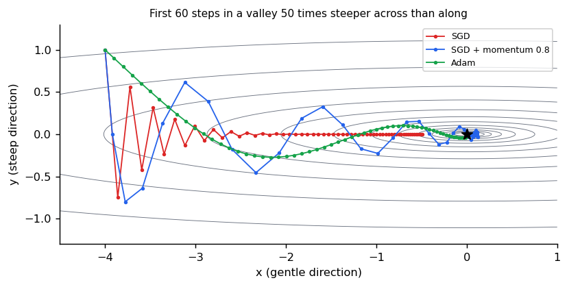
- Momentum keeps a running average of past gradients, so consistent directions build up speed and oscillating ones cancel.
- Adam (1412.6980) also divides each parameter's step by a running estimate of its gradient's size, so steep and flat directions get comparable steps. It is the default for transformers; AdamW, its variant with decoupled weight decay, is what most papers in the tutorial use.
The learning rate is the most important setting in practice. Too high and the loss diverges; too low and nothing happens in your budget. Large runs ramp it up at the start (warmup) and decay it towards the end (the Training at scale module).
6. Generalisation: overfitting and how to spot it
A model is useful only on data it has not seen. Split the data into training (to fit), a validation set (to choose settings and when to stop) and a test set (touched once, at the end). The classic picture: as capacity grows, training error keeps falling, but test error falls and then rises, because a flexible enough model fits the noise as well as the signal:
def polynomial_errors(
    degree: int, n_train: int = 15, noise: float = 0.2, seed: int = 0
) -> tuple[float, float]:
    """Fits a polynomial to noisy samples of sin(3x); returns train and test MSE."""
    generator = torch.Generator().manual_seed(seed)
    x_train = torch.rand(n_train, generator=generator) * 2 - 1
    y_train = torch.sin(3 * x_train) + noise * torch.randn(n_train, generator=generator)
    x_test = torch.linspace(-1, 1, 400)
    y_test = torch.sin(3 * x_test)

    def features(x: torch.Tensor) -> torch.Tensor:
        return torch.stack([x**k for k in range(degree + 1)], dim=1).double()

    coefficients = torch.linalg.lstsq(
        features(x_train), y_train.double()[:, None]
    ).solution
    train = ((features(x_train) @ coefficients).squeeze(1) - y_train.double()) ** 2
    test = ((features(x_test) @ coefficients).squeeze(1) - y_test.double()) ** 2
    return train.mean().item(), test.mean().item()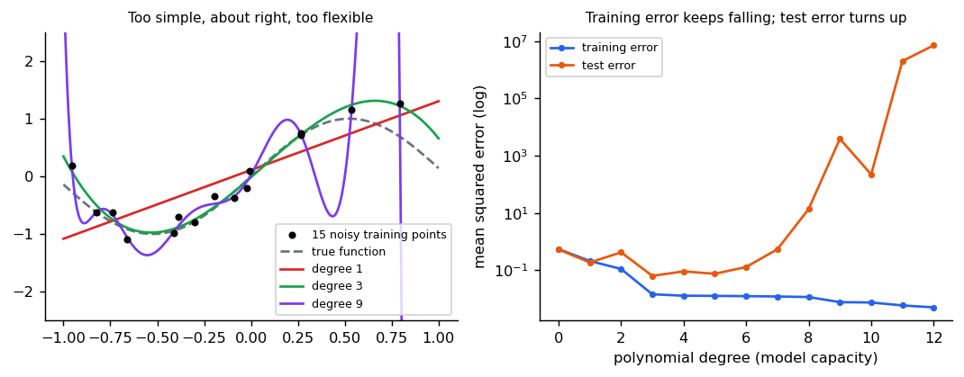
Remedies, each of which appears later in the tutorial:
- More data, the most reliable one (Scaling laws and data recipes).
- Weight decay: penalise large weights.
- Dropout: randomly zero activations during training so no unit can be relied on alone.
- Early stopping: keep the checkpoint with the best validation score.
- Data augmentation: train on transformed copies (crops, colour changes, domain randomisation in Sim-to-real).
Large modern models complicate the classic picture, since very large models trained on enough data keep improving on held-out data, but the discipline of a held-out set never changes.
7. Normalisation and residual connections
Two pieces make deep networks trainable, and both are in every transformer block:
- Normalisation rescales activations to a standard range. Layer normalisation normalises each example's features to zero mean and unit variance and then applies a learned scale and shift; it does not depend on the batch, which suits sequences and small batches.
- Residual connections add a block's input to its output, , so information and gradients have a direct path through a deep stack (Transformers).
8. Embeddings
An embedding is a learned vector standing for a discrete item: a token id, a class, a camera index. It is a lookup table with one row per item, trained like any weight. Embeddings turn integers, which a network cannot use directly, into points in a space where similar items can end up close together. Transformers embed text tokens, image patches (through a linear layer) and positions, and VLAs often embed discretised actions the same way.
9. A small probability toolkit
The generative modules use a handful of quantities repeatedly:
- A distribution assigns probability to outcomes; a Gaussian is described by its mean and standard deviation.
- The expectation is the average of under the distribution, estimated in practice by averaging over samples.
- Entropy : the average surprise of samples from . A fair coin has nats.
- Cross-entropy : the average surprise when the data come from but you score them with a model . Training a classifier minimises exactly this.
- KL divergence : the extra surprise from using instead of . It is zero only when , and it is not symmetric.
def entropy(p: torch.Tensor) -> float:
    """H(p) = -sum p log p, in nats: the average surprise of samples from p."""
    nonzero = p[p > 0]
    return -(nonzero * nonzero.log()).sum().item()


def cross_entropy(p: torch.Tensor, q: torch.Tensor) -> float:
    """H(p, q) = -sum p log q: the average surprise of samples from p under model q."""
    return -(p * q.log()).sum().item()


def kl_divergence(p: torch.Tensor, q: torch.Tensor) -> float:
    """KL(p || q) = H(p, q) - H(p): the extra surprise from using q instead of p."""
    return cross_entropy(p, q) - entropy(p)
The identity "cross-entropy = entropy + KL" (checked in a test) explains why minimising cross-entropy fits a model to data: the entropy of the data is fixed, so lowering cross-entropy lowers the KL. KL divergence then reappears as the VAE's regulariser (Variational autoencoders), the penalty that keeps RLHF close to its starting model (RL for alignment) and the distillation loss (Distillation).
10. Reading the tutorial's code
The reference code is plain PyTorch. Nearly every training loop has the same five lines:
for step in range(steps):
    loss = loss_fn(model(inputs), targets)  # forward pass and loss
    optimizer.zero_grad()                   # clear old gradients
    loss.backward()                         # backpropagation
    optimizer.step()                        # gradient-descent update
Models subclass nn.Module and define forward. torch.no_grad() marks code that does not need
gradients (evaluation, sampling). Seeds are fixed with torch.manual_seed so the quoted numbers
reproduce. Every module's code lives in libs/tutorial/, with tests in libs/tutorial/tests/, and
uv run --group tutorial python -m libs.tutorial.<name> runs its demo.
Reference implementation (PyTorch)
libs/tutorial/basics.py; tests are in libs/tutorial/tests/test_basics.py: hand-written backprop
matches autograd; stable cross-entropy survives logits of 1000 and matches PyTorch's; momentum and Adam
beat plain SGD by more than five times in the narrow valley; more capacity lowers training error while
test error first falls and then rises tenfold; and cross-entropy equals entropy plus KL. Run
uv run --group tutorial python -m libs.tutorial.basics.
Self-test
If you miss more than one, spend an hour on the sections above, or on a standard deep-learning introduction, first.
Quiz
Answer each question; feedback appears as soon as you choose.
Where next
Start with Transformers.
Sources
- Kingma and Ba, Adam: A Method for Stochastic Optimization, 2014.
Capstone: ship a car-following driver
The course capstone: design a teacher that respects a safety envelope, train a driver by imitation, put the RSS filter in front of it, evaluate it on held-out scenarios and write the safety case.
Transformers
Self-attention, multiple heads, positions, the full block, masks and decoding, built up step by step with figures, a hand-checkable example and a tiny trained model.