Variational autoencoders
From autoencoders to VAEs: the latent-variable view, the ELBO, the closed-form KL, the reparameterisation trick, the beta trade-off and posterior collapse, with runnable code.
From autoencoder to VAE
An autoencoder compresses an input x to a small code z and reconstructs it. Nothing makes the space of codes smooth or sampleable: decoding a random z often gives garbage.
A variational autoencoder fixes this by making the encoder output a distribution over z (a mean and a variance), sampling z from it, decoding, and adding a penalty that keeps those distributions close to a simple prior, usually a standard Gaussian. After training you can sample z from the prior and decode to get new data. The rest of this page explains where that recipe comes from and what each part does. Kingma and Welling's An Introduction to Variational Autoencoders is the long-form reference; Doersch's Tutorial on Variational Autoencoders is a gentler walk-through.
The latent-variable view and the ELBO
Suppose the data was made by first drawing a hidden z from a prior , then drawing x from a decoder . Training would maximise the likelihood of the data, . That integral over every possible z has no closed form for a neural-network decoder, and the posterior we would need to evaluate it is just as intractable.
The VAE gets around this with a second network, the encoder, that outputs an approximate posterior . For any such the log-likelihood is bounded below by the evidence lower bound (ELBO):
Maximising the bound trains the decoder and the encoder together. With a Gaussian decoder of fixed variance, the first term is (up to constants) the squared reconstruction error, which gives the loss we use:
- The first term says: the code must carry enough information to rebuild x.
- The KL term says: codes must stay near the prior, so the space is smooth and sampleable.
With this is the negative ELBO. A different is the "beta-VAE" weighting discussed below.
The KL term has a closed form
For a diagonal Gaussian against the standard normal prior, no sampling is needed:
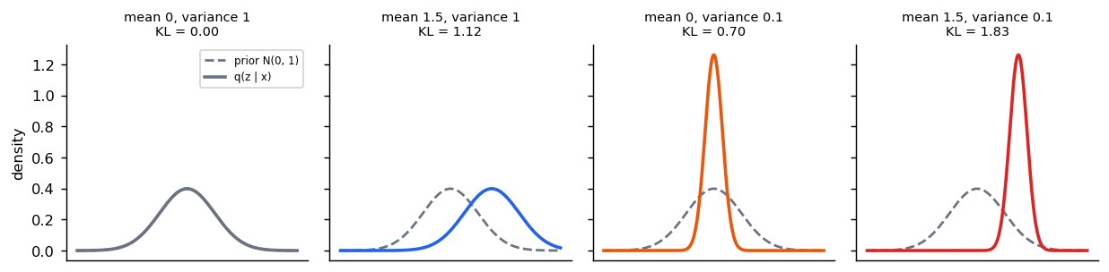
It is zero only when the mean is 0 and the variance is 1 in every dimension, and it grows as the posterior moves away from the prior or gets sharper.
def gaussian_kl(mean: torch.Tensor, log_var: torch.Tensor) -> torch.Tensor:
    """KL(N(mean, exp(log_var)) || N(0, I)) per example, summed over latent dimensions.

    For a diagonal Gaussian against the standard normal this has a closed form:
    0.5 * sum(mean^2 + variance - 1 - log variance). It is zero only when the mean is 0
    and the variance is 1 in every dimension.
    """
    return 0.5 * (mean**2 + log_var.exp() - 1 - log_var).sum(dim=-1)


def elbo_terms(
    x: torch.Tensor, recon: torch.Tensor, mean: torch.Tensor, log_var: torch.Tensor
) -> tuple[torch.Tensor, torch.Tensor]:
    """The two parts of the negative ELBO, averaged over the batch.

    Returns:
        The reconstruction error (distortion) and the KL to the prior (rate).
    """
    distortion = ((recon - x) ** 2).sum(dim=-1).mean()
    return distortion, gaussian_kl(mean, log_var).mean()


def vae_loss(
    x: torch.Tensor,
    recon: torch.Tensor,
    mean: torch.Tensor,
    log_var: torch.Tensor,
    beta: float = 1.0,
) -> torch.Tensor:
    """Negative ELBO: reconstruction error plus beta times KL(q(z|x) || N(0, I))."""
    distortion, rate = elbo_terms(x, recon, mean, log_var)
    return distortion + beta * rate
Tests (libs/tutorial/tests/test_vae.py) check the closed form against a Monte Carlo estimate of
with 200,000 samples, that the KL is zero only at the prior, and that
the loss is the distortion plus beta times the rate.
The reparameterisation trick
Sampling z is not differentiable. Write with . Now the randomness is an input and gradients flow to mean and std. Rezende et al. (1401.4082) describe a closely related backpropagation method for stochastic variables in the same period.
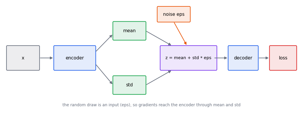
A quick check that it gives the right gradient: for we know , whose derivative with respect to is . The test averages the gradient through 200,000 reparameterised samples (with ) and gets 3.0 within 0.02.
The beta trade-off: rate versus distortion
Think of z as a channel. The KL term is the rate, how much information the code stores about x. The reconstruction error is the distortion. Raising makes information more expensive, so the model stores less of it. Burgess et al. (1804.03599) analyse the beta-VAE objective through exactly this rate-distortion lens.
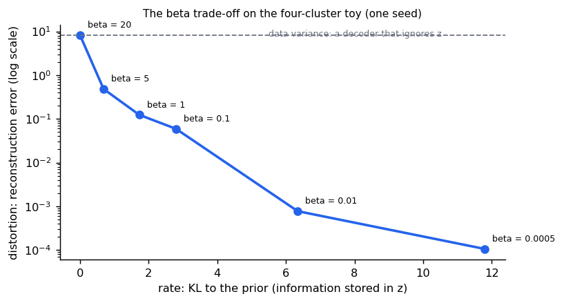
The numbers behind the figure, as mean ± standard deviation over 3 seeds
(uv run --group tutorial python scripts/tutorial_results.py vae reproduces them; the data's total variance, which
a decoder that ignores z cannot beat, is 8.10):
| beta | Rate (KL) | Distortion (reconstruction error) |
|---|---|---|
| 0.0005 | 12.32 ± 0.42 | 0.000 ± 0.000 |
| 0.01 | 6.40 ± 0.04 | 0.001 ± 0.000 |
| 0.1 | 3.05 ± 0.31 | 0.045 ± 0.019 |
| 1 | 1.78 ± 0.05 | 0.121 ± 0.003 |
| 5 | 0.70 ± 0.03 | 0.468 ± 0.029 |
| 20 | 0.00 ± 0.00 | 8.131 ± 0.032 |
Posterior collapse
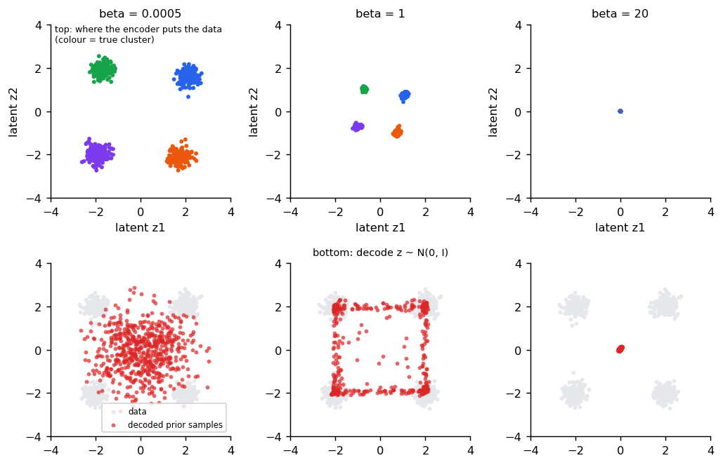
The last row is posterior collapse: the KL is driven to zero, so equals the prior for every x, and the decoder, which gets no information from z, can only output the average of the data. Its error (8.13) equals the data variance (8.10). In our toy this happens only at a large beta, but it is a general failure mode whenever the KL term is cheap to satisfy and the decoder is strong enough to model the data without z. Lowering beta, or raising it gradually from a small value, are common remedies.
The two ends of the sweep also show up in samples. The figure below, from the earlier toy, shows where the encoder puts the four clusters and what the decoder produces from random prior samples at three values of beta.
Where VAEs appear in robot learning
- ACT (the Imitation learning module) uses a conditional VAE during training: a style variable z summarises the demonstration's whole action sequence so the decoder can explain variation between demonstrations. At test time z is set to zero.
- Image and video tokenisers often use a VAE-style autoencoder so that a diffusion or flow model can work in a compact latent space instead of pixels, and their discrete cousins (VQ-VAE and FSQ) are covered in the Discrete tokenizers module.
- World models such as Ha and Schmidhuber's learn a compressed representation of the environment with a VAE (the World models module).
- A VAE has a fast, single-pass decoder, which is its advantage over diffusion. Its weakness is blurry samples when the decoder is simple.
Reference implementation (PyTorch)
Tests are in libs/tutorial/tests/test_vae.py. Run uv run --group tutorial python -m libs.tutorial.vae to train at two
values of beta and compare how close decoded prior samples land to the data.
class VAE(nn.Module):
    """MLP encoder to a Gaussian over the latent, MLP decoder back to the input."""

    def __init__(
        self, input_dim: int = 2, latent_dim: int = 2, hidden: int = 64
    ) -> None:
        """Creates the encoder and decoder."""
        super().__init__()
        self.encoder = nn.Sequential(
            nn.Linear(input_dim, hidden), nn.ReLU(), nn.Linear(hidden, 2 * latent_dim)
        )
        self.decoder = nn.Sequential(
            nn.Linear(latent_dim, hidden), nn.ReLU(), nn.Linear(hidden, input_dim)
        )

    def encode(self, x: torch.Tensor) -> tuple[torch.Tensor, torch.Tensor]:
        """Returns the mean and log-variance of q(z | x)."""
        mean, log_var = self.encoder(x).chunk(2, dim=-1)
        return mean, log_var

    def forward(
        self, x: torch.Tensor
    ) -> tuple[torch.Tensor, torch.Tensor, torch.Tensor]:
        """Returns the reconstruction, mean and log-variance."""
        mean, log_var = self.encode(x)
        # Reparameterisation: the randomness is an input, so gradients reach mean/std.
        z = mean + torch.exp(0.5 * log_var) * torch.randn_like(mean)
        return self.decoder(z), mean, log_var
Check yourself
- What would happen to sampling quality if the KL term were removed?
- What does the reparameterisation trick change, and what does it keep the same?
- In ACT, why is the latent only used in training?
- Why does the VAE maximise a lower bound on the log-likelihood and not the log-likelihood itself?
- What are "rate" and "distortion" in a VAE, and which way does raising beta move each?
- What is posterior collapse, and how can you recognise it from the numbers?
Quiz
Answer each question; feedback appears as soon as you choose.
Sources
- Kingma and Welling, Auto-Encoding Variational Bayes, 2013.
- Kingma and Welling, An Introduction to Variational Autoencoders, 2019.
- Rezende et al., Stochastic Backpropagation and Approximate Inference in Deep Generative Models, 2014.
- Doersch, Tutorial on Variational Autoencoders, 2016.
- Burgess et al., Understanding disentangling in beta-VAE, 2018.
- Zhao et al., Learning Fine-Grained Bimanual Manipulation with Low-Cost Hardware, 2023 (ACT; its CVAE).
Tokens, ViT and VLMs
How text and images become one token sequence: subword tokenizers (BPE), patch embeddings, CLIP and SigLIP, and a vision-language model built from them, with runnable code.
Discrete tokenizers: VQ-VAE and FSQ
How continuous images and actions become a vocabulary of tokens: vector quantization and its training tricks, dead codes and how to measure and fix them, finite scalar quantization, and action tokenizers from per-step bins to FAST-style frequency coding.