Reinforcement learning from scratch
A beginner's path through RL: agents, rewards, returns, values, the Bellman equation, dynamic programming, Monte Carlo and TD learning, Q-learning and SARSA, exploration, DQN and policy gradients, with code you can run.
Why this module
The later modules use RL words freely: policy, return, advantage, baseline, value network, on-policy,
KL penalty. If those are new, start here. This module assumes only what the rest of the tutorial
assumes (you can train a small network with gradient descent) and builds RL up from one small grid
world you can print in a terminal. Every number on this page comes from code in
libs/tutorial/rl_basics.py and can be reproduced with
uv run --group tutorial python scripts/tutorial_results.py rl_basics rl_basics_more.
The path through the page:
- The setting: agents, rewards, returns and the discount (sections 1 and 2).
- Knowing the rules: values, the Bellman equation, value and policy iteration (sections 3 to 5).
- Learning from experience: Monte Carlo, TD, Q-learning and SARSA (sections 6 to 8).
- Exploration (section 9).
- Scaling up: neural networks (DQN) and learning the policy directly (sections 10 and 11).
Afterwards, Reinforcement learning for policies and reasoning covers PPO and GRPO, and RL for alignment covers RLHF.
1. Learning from consequences
Supervised learning has an answer key: for every input, a label says what the output should have been. Reinforcement learning has no answer key. An agent tries something, the world responds, and a single number, the reward, says how good the result was. The agent has to work out which of its choices earned that reward and do more of them.
Think of learning a video game without a manual. Nobody tells you the right button for each frame; you see the score go up or down, sometimes long after the move that caused it.
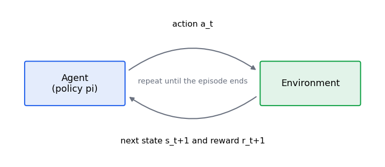
| Word | Meaning | In the grid world below | In a driving VLA |
|---|---|---|---|
| State | What the agent knows now | Which cell it is in | Camera frames, route, ego speed |
| Action | What it can do | Up, right, down, left | A trajectory (or a token of one) |
| Reward | A number scoring one step | +1 goal, −1 pit, −0.04 per step | Progress, no collision, comfort |
| Policy | The agent's rule for choosing actions | An arrow per cell | The model itself |
| Episode | One run from start to end | Start cell to goal or pit | One scenario |
| Return | Total (discounted) reward of an episode | Sum of step rewards | Score of a driven scenario |
Three things make RL harder than supervised learning:
- Credit assignment. The reward may arrive long after the action that deserves it. A car that merges too late is penalised when the lane ends, several seconds after the decision that caused it.
- The data depends on you. The agent only sees the states its own policy leads to. A bad policy never visits the good parts of the world, so it cannot learn about them.
- Exploration. To find better actions the agent must sometimes try actions it believes are worse.
2. The return and the discount
The agent maximises the return, the sum of rewards from now on, with later rewards discounted by a factor between 0 and 1:
With , a reward of 10 three steps away is worth now (the first reward is not discounted). Discounting keeps the sum finite for long episodes, and makes the agent prefer getting a reward sooner.
def discounted_return(rewards: list[float], gamma: float) -> float:
    """The return G = r_0 + gamma r_1 + gamma^2 r_2 + ...

    Raises:
        ValueError: If ``gamma`` is outside [0, 1].
    """
    if not 0.0 <= gamma <= 1.0:
        raise ValueError(f"gamma must be in [0, 1], got {gamma}")
    total = 0.0
    for reward in reversed(rewards):
        total = reward + gamma * total
    return total
A useful rule of thumb: the agent effectively looks about steps ahead. is a horizon of about 2 steps, about 10, about 100. In the grid world below the goal is five steps from the start, so the choice matters:
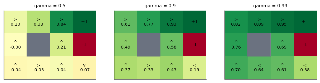
| Effective horizon | Value of the start cell | |
|---|---|---|
| 0.5 | about 2 steps | −0.044 |
| 0.9 | about 10 steps | 0.374 |
| 0.99 | about 100 steps | 0.698 |
With the +1 five steps away is worth now, less than the step costs on the way, so the start cell is worth slightly less than nothing. The cell beside the pit stops trying altogether: bumping into the wall costs −0.04 a step but never risks the pit. is a design choice, not a detail, and in driving it sets how far ahead the planner cares.
3. A world with rules: the grid world
The reference code has the classic textbook grid: 3 rows by 4 columns, a wall in the middle, a goal worth +1, a pit worth −1, and −0.04 for every other step so that dawdling costs something. Moves are slippery: 80 percent of the time the agent goes where it intended, and 10 percent of the time to each side (never backwards). Bumping into a wall or the edge leaves it where it was.
@dataclass(frozen=True)
class GridWorld:
    """A small grid: reach the goal (+1), avoid the pit (-1), every step costs a bit.

    With probability ``slip`` the agent moves to one side of the intended direction
    instead (half to each side). Bumping into a wall or the edge leaves it in place.

    Attributes:
        rows: Grid height.
        cols: Grid width.
        start: Starting cell.
        goal: Terminal cell with reward +1.
        pit: Terminal cell with reward -1.
        walls: Cells that cannot be entered.
        step_reward: Reward for every non-terminal step.
        slip: Probability of moving sideways.
    """

    rows: int = 3
    cols: int = 4
    start: Cell = (2, 0)
    goal: Cell = (0, 3)
    pit: Cell = (1, 3)
    walls: frozenset[Cell] = field(default_factory=lambda: frozenset({(1, 1)}))
    step_reward: float = -0.04
    slip: float = 0.2

    def cells(self) -> list[Cell]:
        """Every cell the agent can be in, walls excluded."""
        return [
            (r, c)
            for r in range(self.rows)
            for c in range(self.cols)
            if (r, c) not in self.walls
        ]

    def is_terminal(self, cell: Cell) -> bool:
        """True for the goal and the pit."""
        return cell in (self.goal, self.pit)

    def _move(self, cell: Cell, action: int) -> Cell:
        dr, dc = ACTIONS[action]
        target = (cell[0] + dr, cell[1] + dc)
        inside = 0 <= target[0] < self.rows and 0 <= target[1] < self.cols
        return target if inside and target not in self.walls else cell

    def _reward(self, cell: Cell) -> float:
        if cell == self.goal:
            return 1.0
        if cell == self.pit:
            return -1.0
        return self.step_reward

    def transitions(self, cell: Cell, action: int) -> list[tuple[float, Cell, float]]:
        """Every outcome of ``action`` in ``cell`` as (probability, next, reward)."""
        outcomes = [(1.0 - self.slip, action)]
        outcomes += [
            (self.slip / 2, (action + 1) % 4),
            (self.slip / 2, (action + 3) % 4),
        ]
        result = []
        for probability, actual in outcomes:
            if probability > 0:
                after = self._move(cell, actual)
                result.append((probability, after, self._reward(after)))
        return result

    def step(self, cell: Cell, action: int, rng: random.Random) -> tuple[Cell, float]:
        """Samples one transition."""
        draw, total = rng.random(), 0.0
        outcomes = self.transitions(cell, action)
        for probability, after, reward in outcomes:
            total += probability
            if draw < total:
                return after, reward
        return outcomes[-1][1], outcomes[-1][2]
This is a Markov decision process (MDP): states, actions, rewards, and transition probabilities that depend only on the current state and action, not on the history. That "only the present matters" assumption is the Markov property. A driving scene from one camera frame is not Markov (you cannot see velocities in one frame), which is one reason driving models take several frames and the ego state as input.
4. Values and the Bellman equation
A value function answers "how much return do I expect from here?":
- : expected return starting in state and following policy .
- : expected return taking action in , then following . If you know , the best action is simply the one with the largest .
The key fact about values is the Bellman equation: the value of a state is the reward you get now plus the discounted value of where you land. For the best possible policy:
Read it as: try each action, average over where you might slip to, and keep the best.
A worked example you can check by hand
Take the cell just left of the goal, (0, 2), once the values have settled (the right-hand grid of the figure in section 5). Pressing right has three outcomes:
| Outcome | Probability | Reward | Value of where you land | |
|---|---|---|---|---|
| Reach the goal | 0.8 | +1 | 0 (the episode ends) | 0.800 |
| Slip down to (1, 2) | 0.1 | −0.04 | 0.641 | 0.057 |
| Slip up, bump the edge, stay | 0.1 | −0.04 | 0.942 | 0.085 |
| Total | 0.942 |
Doing the same for the other actions gives up 0.860, down 0.631 and left 0.745. Right is best, and its total is exactly the cell's value, 0.942: the equation holds. A test checks it for every cell.
Value iteration: let the equation do the work
Value iteration starts with every value at zero and applies the Bellman equation to every cell, over and over (each pass is a sweep), until nothing changes. On the first sweep only the cell next to the goal sees anything good: . On the second sweep its neighbours see that 0.79, and so on: the good news spreads outward from the goal one step per sweep.

def action_values(
    world: GridWorld, values: dict[Cell, float], cell: Cell, gamma: float
) -> list[float]:
    """One-step lookahead: expected r + gamma V(s') for each action in ``cell``."""
    return [
        sum(
            p * (r + gamma * values[after])
            for p, after, r in world.transitions(cell, a)
        )
        for a in range(len(ACTIONS))
    ]


def bellman_sweep(
    world: GridWorld, values: dict[Cell, float], gamma: float
) -> dict[Cell, float]:
    """Applies the Bellman optimality equation once to every cell (from old values)."""
    updated = dict.fromkeys(world.cells(), 0.0)
    for cell in world.cells():
        if not world.is_terminal(cell):
            updated[cell] = max(action_values(world, values, cell, gamma))
    return updated


def value_iteration(
    world: GridWorld, gamma: float = 0.95, tolerance: float = 1e-8
) -> dict[Cell, float]:
    """Solves the Bellman optimality equation by repeating it until it stops changing.

    V(s) = max_a sum_s' P(s' | s, a) [r + gamma V(s')], with V = 0 at terminal cells.

    Returns:
        The optimal value of every cell.
    """
    values = dict.fromkeys(world.cells(), 0.0)
    while True:
        updated = bellman_sweep(world, values, gamma)
        change = max(abs(updated[c] - values[c]) for c in values)
        values = updated
        if change < tolerance:
            return values


def greedy_from_values(
    world: GridWorld, values: dict[Cell, float], gamma: float = 0.95
) -> dict[Cell, int]:
    """The action with the best one-step lookahead in every non-terminal cell."""
    policy = {}
    for cell in world.cells():
        if not world.is_terminal(cell):
            scores = action_values(world, values, cell, gamma)
            policy[cell] = max(range(len(ACTIONS)), key=scores.__getitem__)
    return policy
Value iteration needs the transition probabilities, so it is planning with a known model, not learning. That family of methods is called dynamic programming.
5. Policy evaluation and policy iteration
Value iteration mixes two questions: "how good is this policy?" and "can I do better?". Separating them gives a second classic algorithm.
- Policy evaluation: for a fixed policy, repeat until it settles. No max: just follow the policy.
- Policy improvement: in every cell, switch to the action with the best lookahead under those values (act greedily).
- Policy iteration: alternate the two until the policy stops changing.
def policy_evaluation(
    world: GridWorld,
    policy: dict[Cell, list[float]],
    gamma: float = 0.95,
    tolerance: float = 1e-8,
) -> dict[Cell, float]:
    """V of a fixed policy: repeat V(s) = sum_a pi(a|s) [lookahead] until stable.

    Args:
        world: The grid world.
        policy: Action probabilities for every non-terminal cell.
        gamma: Discount factor.
        tolerance: Stop when no value changes by more than this.
    """
    values = dict.fromkeys(world.cells(), 0.0)
    while True:
        updated = dict.fromkeys(world.cells(), 0.0)
        for cell in policy:
            lookahead = action_values(world, values, cell, gamma)
            updated[cell] = sum(
                p * v for p, v in zip(policy[cell], lookahead, strict=True)
            )
        change = max(abs(updated[c] - values[c]) for c in values)
        values = updated
        if change < tolerance:
            return values


def policy_iteration(
    world: GridWorld, gamma: float = 0.95
) -> list[tuple[dict[Cell, int], dict[Cell, float]]]:
    """Evaluate, act greedily on the values, repeat until the policy stops changing.

    Starts from the uniformly random policy.

    Returns:
        The greedy policy and the values it was derived from, for every round.
    """
    uniform = [1 / len(ACTIONS)] * len(ACTIONS)
    probs = {c: uniform for c in world.cells() if not world.is_terminal(c)}
    history: list[tuple[dict[Cell, int], dict[Cell, float]]] = []
    while True:
        values = policy_evaluation(world, probs, gamma)
        greedy = greedy_from_values(world, values, gamma)
        if history and greedy == history[-1][0]:
            return history
        history.append((greedy, values))
        probs = {
            c: [1.0 if a == greedy[c] else 0.0 for a in range(len(ACTIONS))]
            for c in greedy
        }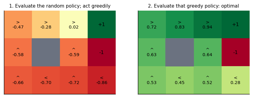
The random policy's values are bad, yet they rank the actions correctly. That is the general lesson behind every actor-critic method later on: values do not have to be accurate to improve a policy, they only have to point in the right direction.
6. Learning from experience: Monte Carlo versus temporal difference
Usually you do not have : nobody gives you the physics of traffic. You have to learn from episodes. The first question is prediction: given a fixed policy, estimate its values from experience.
- Monte Carlo (MC): play the episode to the end, then move each visited state's value toward the return that actually followed: . Unbiased, but a whole episode's worth of randomness lands in every update.
- Temporal difference, TD(0): after every single step, move toward a one-step guess, . It uses its own estimate of the next state, which is called bootstrapping. Less noisy, but biased while that estimate is still wrong.
def prediction_errors(
    world: GridWorld,
    policy: dict[Cell, int],
    *,
    method: str,
    episodes: int = 300,
    alpha: float = 0.05,
    gamma: float = 0.95,
    seed: int = 0,
) -> list[float]:
    """Learns V of a fixed policy from episodes; returns RMS error after each episode.

    Each episode starts in a random cell, so every state keeps being visited.
    ``"mc"`` (Monte Carlo) waits for the episode to end and moves V(s_t) toward the
    actual return G_t. ``"td"`` (TD(0)) moves V(s_t) toward r + gamma V(s_t+1) right
    after each step, using its own current estimate of the next state (bootstrapping).

    Raises:
        ValueError: If ``method`` is not ``"mc"`` or ``"td"``.
    """
    if method not in ("mc", "td"):
        raise ValueError(f"method must be 'mc' or 'td', got {method!r}")
    probs = {c: [1.0 if a == policy[c] else 0.0 for a in range(4)] for c in policy}
    truth = policy_evaluation(world, probs, gamma)
    rng = random.Random(seed)
    values = dict.fromkeys(world.cells(), 0.0)
    live = [c for c in world.cells() if not world.is_terminal(c)]
    errors = []
    for _ in range(episodes):
        cell, visited = rng.choice(live), []
        for _ in range(200):
            after, reward = world.step(cell, policy[cell], rng)
            if method == "td":
                values[cell] += alpha * (reward + gamma * values[after] - values[cell])
            visited.append((cell, reward))
            cell = after
            if world.is_terminal(cell):
                break
        if method == "mc":
            ret = 0.0
            for state, reward in reversed(visited):
                ret = reward + gamma * ret
                values[state] += alpha * (ret - values[state])
        squared = [(values[c] - truth[c]) ** 2 for c in live]
        errors.append((sum(squared) / len(squared)) ** 0.5)
    return errors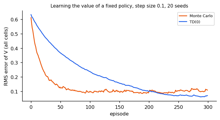
| Episodes | Monte Carlo RMS error | TD(0) RMS error |
|---|---|---|
| 10 | 0.386 | 0.565 |
| 50 | 0.130 | 0.370 |
| 300 | 0.108 | 0.070 |
The trade-off in one picture. MC learns faster at first here: it sees real returns immediately, while TD has to pass value back one step per visit. But MC keeps jittering, because every update carries the noise of an entire episode's slips; TD's updates carry one step's noise and it ends lower. In long or never-ending tasks, waiting for the end of the episode is not even possible, which is why most practical RL (DQN, PPO's critic, GAE) is built on TD-style bootstrapping.
7. Q-learning: TD for choosing actions
Q-learning applies the TD idea to action values, and learns the best policy while following an exploratory one. After every step:
The bracket is the TD error: how surprised the agent was. The agent acts epsilon-greedily: usually the best-looking action, but a random one with probability so that it keeps exploring.
def _epsilon_greedy(values: list[float], epsilon: float, rng: random.Random) -> int:
    if rng.random() < epsilon:
        return rng.randrange(len(values))
    return max(range(len(values)), key=values.__getitem__)


def q_learning(
    world: Environment,
    *,
    episodes: int = 3000,
    alpha: float = 0.1,
    epsilon: float = 0.1,
    gamma: float = 0.95,
    seed: int = 0,
    trace: list[tuple[Cell, int, float, Cell, float, float, float]] | None = None,
) -> tuple[dict[Cell, list[float]], list[float]]:
    """Learns action values from experience, without knowing the transition rules.

    After each step: Q(s, a) += alpha * (r + gamma * max_a' Q(s', a') - Q(s, a)).
    Actions are epsilon-greedy: random with probability ``epsilon``, else the best.

    Args:
        world: Any environment with ``start``, ``cells``, ``is_terminal`` and ``step``.
        episodes: Number of episodes (each capped at 200 steps).
        alpha: Step size.
        epsilon: Exploration probability.
        gamma: Discount factor.
        seed: Seed for exploration and slips.
        trace: If given, every update is appended as (state, action, reward, next
            state, old Q value, TD target, new Q value).

    Returns:
        The Q table and the undiscounted return of every episode.
    """
    rng = random.Random(seed)
    q = {cell: [0.0] * len(ACTIONS) for cell in world.cells()}
    returns = []
    for _ in range(episodes):
        cell, total = world.start, 0.0
        for _ in range(200):
            action = _epsilon_greedy(q[cell], epsilon, rng)
            after, reward = world.step(cell, action, rng)
            target = reward
            if not world.is_terminal(after):
                target += gamma * max(q[after])
            old = q[cell][action]
            q[cell][action] = old + alpha * (target - old)
            if trace is not None:
                trace.append(
                    (cell, action, reward, after, old, target, q[cell][action])
                )
            cell, total = after, total + reward
            if world.is_terminal(cell):
                break
        returns.append(total)
    return q, returns
Watch the first updates
All values start at 0, with and . Some updates from the first
episodes of seed 0 (the trace argument records them):
| Update | State, action | Reward | Lands in | Old | Target | New |
|---|---|---|---|---|---|---|
| 1 | (2, 0), up | −0.04 | (1, 0) | 0 | −0.04 | −0.004 |
| 8 | (0, 2), right | +1 | goal | 0 | 1 | 0.100 |
| 31 | (0, 1), right | −0.04 | (0, 2) | −0.004 | 0.002 | |
| 32 | (0, 2), right | +1 | goal | 0.100 | 1 | 0.190 |
| 37 | (1, 2), up | −0.04 | (0, 2) | 0 | 0.014 |
Early steps only learn that moving costs 0.04. Once the agent stumbles into the goal (update 8), the cell beside it gets credit, and on later visits its neighbours (updates 31 and 37) borrow that credit through the term. This is credit assignment working backwards one step at a time, the same spreading you saw in value iteration, but driven by experience instead of a model.
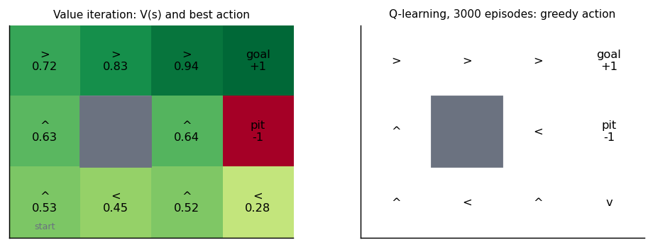
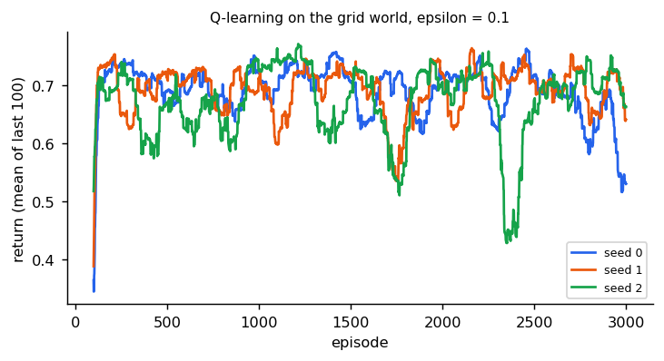
Over 5 seeds, Q-learning's greedy action matched value iteration in 0.89 ± 0.08 of the cells, and the mean return over the last 500 episodes was 0.68 ± 0.03. The cells it gets wrong are ones it rarely visits (in the figure, the cells left of and below the pit): Q-learning only learns about states its own behaviour reaches. That is the "data depends on you" problem from section 1, in miniature.
8. On-policy versus off-policy: SARSA on the cliff
Q-learning's target uses : the value of acting greedily next, even though the agent will actually act epsilon-greedily. It learns about one policy (greedy) while following another (exploratory). That makes it off-policy.
SARSA (named after the tuple state, action, reward, state, action it uses) is the on-policy version: the target uses the action the agent will really take next, exploration included.
def sarsa(
    world: Environment,
    *,
    episodes: int = 3000,
    alpha: float = 0.1,
    epsilon: float = 0.1,
    gamma: float = 1.0,
    seed: int = 0,
) -> tuple[dict[Cell, list[float]], list[float]]:
    """On-policy TD control: the target uses the action the agent will actually take.

    Q(s, a) += alpha * (r + gamma * Q(s', a') - Q(s, a)), where a' is chosen
    epsilon-greedily, exactly as the agent will act. Q-learning uses max_a' instead,
    which learns about the greedy policy while behaving epsilon-greedily.

    Returns:
        The Q table and the undiscounted return of every episode.
    """
    rng = random.Random(seed)
    q = {cell: [0.0] * len(ACTIONS) for cell in world.cells()}
    returns = []
    for _ in range(episodes):
        cell, total = world.start, 0.0
        action = _epsilon_greedy(q[cell], epsilon, rng)
        for _ in range(200):
            after, reward = world.step(cell, action, rng)
            next_action = _epsilon_greedy(q[after], epsilon, rng)
            target = reward
            if not world.is_terminal(after):
                target += gamma * q[after][next_action]
            q[cell][action] += alpha * (target - q[cell][action])
            cell, action, total = after, next_action, total + reward
            if world.is_terminal(cell):
                break
        returns.append(total)
    return q, returns


def greedy_path(
    world: Environment, q: dict[Cell, list[float]], limit: int = 60
) -> list[Cell]:
    """Cells visited by following the greedy action from the start (no exploration)."""
    rng = random.Random(0)
    cell, path = world.start, [world.start]
    for _ in range(limit):
        cell, _ = world.step(
            cell, max(range(len(ACTIONS)), key=q[cell].__getitem__), rng
        )
        path.append(cell)
        if world.is_terminal(cell):
            break
    return path
The difference shows on the classic cliff walk: a 4 by 12 grid where the bottom row between start and goal is a cliff. Every step costs −1; stepping off the cliff costs −100 and sends you back to the start.
@dataclass(frozen=True)
class CliffWalk:
    """The classic cliff: walk along the bottom edge without falling off.

    A 4 x 12 grid. The start is the bottom-left cell and the goal the bottom-right; the
    cells between them on the bottom row are a cliff. Every step costs -1; stepping
    onto the cliff costs -100 and sends the agent back to the start. Moves are
    deterministic.
    """

    rows: int = 4
    cols: int = 12
    start: Cell = (3, 0)
    goal: Cell = (3, 11)

    def cells(self) -> list[Cell]:
        """Every cell, cliff included (the agent never rests on it)."""
        return [(r, c) for r in range(self.rows) for c in range(self.cols)]

    def is_cliff(self, cell: Cell) -> bool:
        """True for the bottom-row cells between start and goal."""
        return cell[0] == self.rows - 1 and 0 < cell[1] < self.cols - 1

    def is_terminal(self, cell: Cell) -> bool:
        """Only the goal ends an episode."""
        return cell == self.goal

    def step(self, cell: Cell, action: int, rng: random.Random) -> tuple[Cell, float]:
        """Moves one cell (``rng`` is unused: the cliff is deterministic)."""
        del rng
        dr, dc = ACTIONS[action]
        after = (
            min(max(cell[0] + dr, 0), self.rows - 1),
            min(max(cell[1] + dc, 0), self.cols - 1),
        )
        if self.is_cliff(after):
            return self.start, -100.0
        return after, -1.0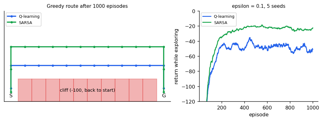
| Method | Greedy route | Return per episode while exploring (last 200 of 1000, 5 seeds) |
|---|---|---|
| Q-learning | Along the cliff edge (13 steps, the shortest) | −51.2 ± 2.7 |
| SARSA | One or two rows above it | −24.8 ± 2.5 |
Which is "right" depends on what you will deploy. Q-learning found the best route for an agent that will stop exploring; but while it explores, a random step next to the cliff often costs −100. SARSA accounts for its own randomness and keeps a safety margin. A robot that will keep some randomness, or a car whose actuation is never exact, is closer to SARSA's assumption.
9. Exploration versus exploitation
The simplest RL problem has one state and several actions: a multi-armed bandit, named after a row of slot machines. Each arm pays a random reward with an unknown mean. Pull the arm that looks best (exploit) or try another to learn more (explore)?
def epsilon_greedy_bandit(
    means: list[float], epsilon: float, steps: int = 1000, seed: int = 0
) -> list[bool]:
    """Plays a Gaussian-reward bandit; returns whether each pull chose the best arm.

    The agent keeps a running average reward per arm. With probability ``epsilon`` it
    explores (a random arm); otherwise it exploits (the arm with the best average).
    """
    rng = random.Random(seed)
    counts = [0] * len(means)
    estimates = [0.0] * len(means)
    best = max(range(len(means)), key=means.__getitem__)
    chose_best = []
    for _ in range(steps):
        if rng.random() < epsilon:
            arm = rng.randrange(len(means))
        else:
            arm = max(range(len(means)), key=estimates.__getitem__)
        reward = rng.gauss(means[arm], 1.0)
        counts[arm] += 1
        estimates[arm] += (reward - estimates[arm]) / counts[arm]
        chose_best.append(arm == best)
    return chose_best
Epsilon-greedy explores blindly: a random arm, even one already known to be bad. Upper confidence bound (UCB) explores where it is still uncertain. Each arm gets a score
where is its average reward so far, how often it was pulled and the total number of pulls. Arms pulled rarely get a large bonus; the bonus shrinks as evidence accumulates. "Optimism in the face of uncertainty."
def ucb_bandit(
    means: list[float], c: float = 1.0, steps: int = 1000, seed: int = 0
) -> list[bool]:
    """Upper confidence bound: pick the arm with the best optimistic estimate.

    Score = average reward + c * sqrt(ln t / pulls). Rarely pulled arms get a large
    bonus, so exploration is directed at arms that might be better, not random.
    """
    rng = random.Random(seed)
    counts = [0] * len(means)
    estimates = [0.0] * len(means)
    best = max(range(len(means)), key=means.__getitem__)
    chose_best = []
    for t in range(1, steps + 1):
        if t <= len(means):
            arm = t - 1
        else:
            scores = [
                estimates[a] + c * math.sqrt(math.log(t) / counts[a])
                for a in range(len(means))
            ]
            arm = max(range(len(means)), key=scores.__getitem__)
        reward = rng.gauss(means[arm], 1.0)
        counts[arm] += 1
        estimates[arm] += (reward - estimates[arm]) / counts[arm]
        chose_best.append(arm == best)
    return chose_best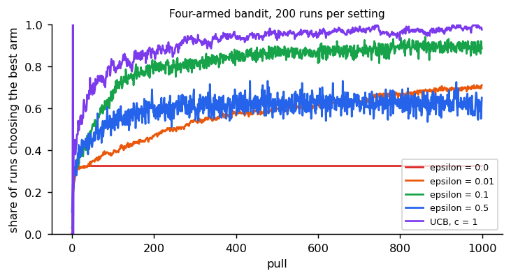
| Strategy | Best arm in the last 200 of 1000 pulls | Best arm over all 1000 pulls |
|---|---|---|
| Epsilon 0 (never explore) | 0.33 | |
| Epsilon 0.01 | 0.69 | |
| Epsilon 0.1 | 0.89 | 0.81 |
| Epsilon 0.5 | 0.62 | |
| UCB, | 0.98 | 0.91 |
Never exploring locks in whichever arm happened to look good first. Exploring too much wastes pulls on arms already known to be bad. Directed exploration (UCB) beats random exploration here. In large problems the same idea appears as optimism bonuses, curiosity rewards, or simply noise added to actions.
10. From tables to networks: deep Q-learning
A table needs one row per state. A camera image has more possible states than atoms in the universe, so real problems replace the table with a network and train it to reduce the TD error. Done naively this is unstable, and DQN (1312.5602), which learned Atari games from raw pixels, is remembered for the ingredients that make it work:
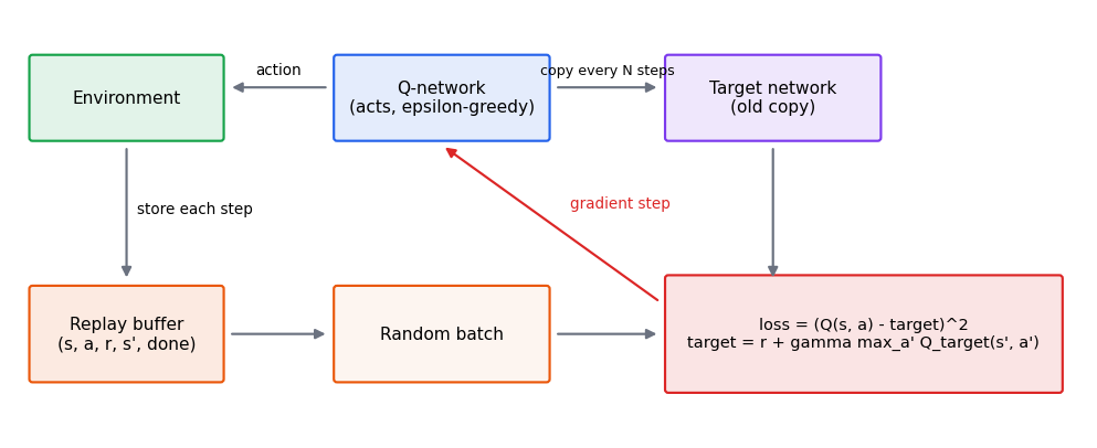
- Replay buffer. Consecutive steps are nearly identical, and training on them in order is like training a classifier on one class at a time. Storing transitions and sampling random batches makes the data closer to independent.
- Target network. The TD target contains itself. If the same network produces the target and is updated toward it, the target moves with every step, like chasing your own shadow. A frozen copy, refreshed every few hundred updates, holds it still.
- Decaying exploration. Start fully random and reduce epsilon as the estimates improve.
def dqn(
    world: GridWorld,
    *,
    episodes: int = 300,
    batch: int = 64,
    gamma: float = 0.95,
    sync_every: int = 100,
    seed: int = 0,
) -> torch.nn.Module:
    """Deep Q-learning on the grid world: a network instead of a table.

    The three ingredients that make Q-learning work with a neural network:

    * a Q-network mapping a state (one-hot cell here; pixels in DQN) to a Q per action;
    * a replay buffer, so each update uses a random batch of old transitions instead of
      the last few, highly correlated ones;
    * a target network, a periodically refreshed copy used for the TD target, so the
      target does not move with every gradient step.

    Exploration decays from fully random to 5 percent over the first half of training.

    Returns:
        The trained Q-network.
    """
    torch.manual_seed(seed)
    rng = random.Random(seed)
    cells = world.cells()
    index = {cell: i for i, cell in enumerate(cells)}
    eye = torch.eye(len(cells))
    net = torch.nn.Sequential(
        torch.nn.Linear(len(cells), 64), torch.nn.ReLU(), torch.nn.Linear(64, 4)
    )
    target_net = copy.deepcopy(net)
    optimizer = torch.optim.Adam(net.parameters(), lr=1e-3)
    buffer: deque[tuple[int, int, float, int, float]] = deque(maxlen=5000)
    updates = 0
    for episode in range(episodes):
        epsilon = max(0.05, 1.0 - episode / (episodes / 2))
        cell = world.start
        for _ in range(100):
            with torch.no_grad():
                q_values = net(eye[index[cell]]).tolist()
            action = _epsilon_greedy(q_values, epsilon, rng)
            after, reward = world.step(cell, action, rng)
            done = float(world.is_terminal(after))
            buffer.append((index[cell], action, reward, index[after], done))
            cell = after
            if len(buffer) >= batch:
                sample = rng.sample(list(buffer), batch)
                s, a, r, s2, d = (torch.tensor(column) for column in zip(*sample))
                with torch.no_grad():
                    best_next = target_net(eye[s2]).max(dim=1).values
                    target = r.float() + gamma * (1 - d.float()) * best_next
                predicted = net(eye[s])[torch.arange(batch), a]
                loss = torch.nn.functional.mse_loss(predicted, target)
                optimizer.zero_grad()
                loss.backward()
                optimizer.step()
                updates += 1
                if updates % sync_every == 0:
                    target_net.load_state_dict(net.state_dict())
            if done:
                break
    return net
On the grid world (state = one-hot cell, 300 episodes), the DQN's greedy action matched the optimal policy in 8, 8 and 9 of the 9 cells over three seeds, about as well as the table. The point is not this world, where the table is fine, but that nothing in the code depends on the state being small.
11. Learning the policy directly: policy gradients
Q-learning learns values and derives a policy from them. That gets awkward when actions are continuous (a steering angle, a whole trajectory): you cannot take a max over infinitely many actions. Policy-gradient methods skip the values and adjust the policy's parameters directly: make actions that led to a high return more likely.
Where the formula comes from
We want the gradient of the expected return . The reward does not depend on , only the probabilities do, so
using (the log-derivative trick). The last form is an average over actions the policy itself samples, so you can estimate it from experience without knowing how the reward is computed. For a whole episode, each action's is weighted by the return that followed it. That is REINFORCE:
Why a baseline
is a baseline, a number subtracted from the return that does not depend on the action. Because , subtracting it does not change the average gradient, but it changes the noise enormously. If every reward is around 5, then without a baseline every action gets pushed up, and only the small difference between actions carries information.
def policy_gradient_samples(
    means: tuple[float, float], baseline: float, samples: int = 5000, seed: int = 0
) -> torch.Tensor:
    """One-sample REINFORCE estimates of d(expected reward)/d(logit of arm 1).

    The policy is a fair coin over two arms (logits 0, 0). Each estimate is
    (reward - baseline) * d log pi(arm) / d logit_1, which is +-0.5 here.

    Returns:
        Shape (samples,): the individual gradient estimates.
    """
    generator = torch.Generator().manual_seed(seed)
    arms = torch.randint(0, 2, (samples,), generator=generator)
    rewards = torch.tensor(means)[arms] + torch.randn(samples, generator=generator)
    score = torch.where(arms == 1, 0.5, -0.5)
    return (rewards - baseline) * score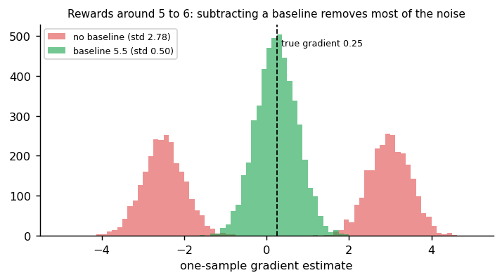
REINFORCE on the grid world
The reference code also runs REINFORCE on the grid world, with a table of action logits per cell, with and without a learned value table as the baseline:
def reinforce(
    world: GridWorld,
    *,
    episodes: int = 600,
    lr: float = 0.1,
    baseline: bool = True,
    gamma: float = 0.95,
    seed: int = 0,
) -> list[float]:
    """REINFORCE on the grid world with a table of action logits per cell.

    After each episode, every visited (s_t, a_t) is pushed by (G_t - b(s_t)) times the
    gradient of log pi(a_t | s_t). With ``baseline``, b is a learned value table moved
    toward the observed returns (a minimal actor-critic); without it, b = 0.

    Returns:
        The undiscounted return of every episode.
    """
    torch.manual_seed(seed)
    rng = random.Random(seed)
    index = {cell: i for i, cell in enumerate(world.cells())}
    logits = torch.zeros(len(index), len(ACTIONS), requires_grad=True)
    optimizer = torch.optim.Adam([logits], lr=lr)
    values = torch.zeros(len(index))
    returns = []
    for _ in range(episodes):
        cell, steps = world.start, []
        for _ in range(100):
            probs = torch.softmax(logits[index[cell]].detach(), dim=0)
            action = int(torch.multinomial(probs, 1))
            after, reward = world.step(cell, action, rng)
            steps.append((index[cell], action, reward))
            cell = after
            if world.is_terminal(cell):
                break
        rows = torch.tensor([s for s, _, _ in steps])
        actions = torch.tensor([a for _, a, _ in steps])
        future, ret = [], 0.0
        for _, _, reward in reversed(steps):
            ret = reward + gamma * ret
            future.append(ret)
        future_t = torch.tensor(future[::-1])
        advantage = future_t - values[rows] if baseline else future_t
        logp = torch.log_softmax(logits[rows], dim=1)[torch.arange(len(steps)), actions]
        loss = -(advantage * logp).sum()
        optimizer.zero_grad()
        loss.backward()
        optimizer.step()
        if baseline:
            values.index_add_(0, rows, 0.1 * (future_t - values[rows]))
        returns.append(sum(r for _, _, r in steps))
    return returns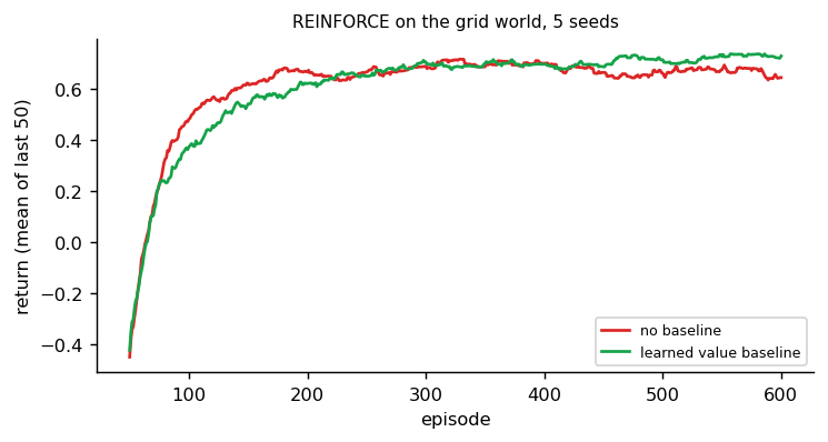
| Return, episodes 50 to 150 | Return, last 100 of 600 | |
|---|---|---|
| No baseline | 0.55 ± 0.04 | 0.66 ± 0.07 |
| Learned value baseline | 0.46 ± 0.17 | 0.73 ± 0.03 |
An honest toy result: the learned baseline starts at zero and is wrong for a while, so early on it can hurt; once it is accurate, updates are less noisy and the policy settles better. Compare REINFORCE's few hundred episodes with Q-learning's: policy gradients are simple and handle any action space, but they are sample-hungry, which is why every practical method adds variance reduction.
is called the advantage: how much better this action did than expected. A policy plus a learned value function as the baseline (the critic) is an actor-critic method. Generalized Advantage Estimation (1506.02438) uses value functions to cut the variance of policy-gradient estimates at the cost of some bias. PPO and GRPO are both answers to the questions "what baseline?" and "how big a step?", covered in the next RL module.
12. A map of RL methods
| Family | Learns | Examples | Where |
|---|---|---|---|
| Dynamic programming | Values from a known model | Value iteration, policy iteration | Sections 4 and 5 |
| Value-based | , acts greedily | Q-learning, SARSA, DQN | Sections 7, 8 and 10 |
| Policy gradient | The policy directly | REINFORCE, PPO, GRPO | Section 11; RL for policies and reasoning |
| Actor-critic | A policy and a value function | REINFORCE with a learned baseline, PPO with a critic | Section 11; same |
| Model-based | A model of the world, then plans | Dreamer | World models |
| Offline | From a fixed log, no new interaction | CQL, IQL | Preference learning and offline RL |
| From human preferences | A reward from comparisons, then RL | RLHF, DPO | RL for alignment |
Three distinctions you will meet everywhere:
- Model-based or model-free: does the method use (or learn) , or only samples?
- On-policy or off-policy: can it learn from data produced by a different (older, more exploratory, human) policy? Q-learning can; SARSA and REINFORCE cannot directly.
- Online or offline: can it interact while learning, or only read a fixed log?
13. What goes wrong in practice
- Reward hacking. The agent maximises the reward you wrote, not the one you meant. In the grid world, a step cost of −2 instead of −0.04 makes the cells next to the pit head straight into it (a test checks this), because ending the episode at −1 beats paying −2 per step; a driving reward that only punishes collisions makes standing still optimal.
- Sparse rewards. If only success is rewarded, a random agent may never see a reward. Reward shaping, demonstrations or curricula help.
- Instability. Bootstrapping from your own estimates (the TD target) and changing data can diverge, which is why practical algorithms clip updates, use target networks or stay close to a reference policy.
- Sample cost. RL needs many episodes, which is cheap in simulation and expensive on a robot. See Sim-to-real.
Reference implementation (PyTorch)
libs/tutorial/rl_basics.py; tests are in libs/tutorial/tests/test_rl_basics.py. They check, among
other things: discounted returns by hand; transition probabilities sum to one and slips never go
backwards; one Bellman sweep by hand; value iteration spreads one cell per sweep and its values
satisfy the Bellman equation; policy evaluation of the optimal policy returns the optimal values and
policy iteration ends at the same policy; a short horizon gives up on the distant goal; the Q-learning
trace follows the update rule; Monte Carlo is ahead early and TD ends lower; SARSA keeps further from
the cliff and earns more while exploring; UCB beats epsilon-greedy on the bandit; the baseline helps
REINFORCE; and DQN learns the main route. Run uv run --group tutorial python -m libs.tutorial.rl_basics to print both
grid-world policies as arrows.
Further reading
- Sutton and Barto, Reinforcement Learning: An Introduction, 2nd edition: the standard textbook, free on the authors' site. Chapters 2 to 6 cover sections 1 to 9 of this page (the cliff walk is one of its examples), and chapter 13 covers policy gradients. The 3 by 4 grid world is the classic example from Russell and Norvig's Artificial Intelligence: A Modern Approach.
- OpenAI, Spinning Up: Key Concepts in RL: the same vocabulary in the deep-RL setting.
Check yourself
- Name two ways RL differs from supervised learning.
- With and rewards 1, 1, 1, what is the return? What horizon does correspond to?
- Redo the worked Bellman example for the action up in cell (0, 2). Where can the agent end up?
- Why does the optimal grid-world policy go left beside the pit?
- Why can acting greedily on the random policy's values already give a good policy?
- Monte Carlo or TD: which uses its own estimates, which waits for the end of the episode, and which was ahead after 10 episodes here?
- Why does Q-learning walk along the cliff edge while SARSA keeps a margin?
- What problems do the replay buffer and the target network solve in DQN?
- Why does subtracting a baseline not change the expected policy gradient, and what does it change?
Quiz
Answer each question; feedback appears as soon as you choose.
Sources
- Sutton and Barto, Reinforcement Learning: An Introduction, 2nd edition, 2018.
- Mnih et al., Playing Atari with Deep Reinforcement Learning, 2013 (DQN).
- Schulman et al., High-Dimensional Continuous Control Using Generalized Advantage Estimation, 2015.
- OpenAI, Spinning Up: Key Concepts in RL.
Imitation learning and action chunking
Behaviour cloning, why it drifts (measured on a lane-keeping toy), DART and DAgger, action chunks and temporal ensembling, and why generative policies help, with our SO-100 measurements.
Reinforcement learning for policies and reasoning
Policy gradients in depth: the advantage and GAE bias-variance dial, PPO's clip and KL penalty (three estimators compared), GRPO's group baseline and its subtle shrinkage, reward design in Alpamayo-R1, and reward hacking.