RL for real robots: sim-to-real
Why policies trained in simulation fail on hardware, and what domain randomization (how wide?), massively parallel training and RMA-style adaptation buy, with a runnable toy, measured trade-offs, and a checklist for driving and robot simulators.
The reality gap
Reinforcement learning needs millions of trials, which only a simulator provides quickly. A policy trained there meets a different world on hardware: masses, friction, motor response, delays, sensor noise and rendering all differ. That mismatch is the reality gap, and closing it is the core of sim-to-real transfer. A survey of the area is 2009.13303.
Main techniques
- Domain randomization (1703.06907). Randomize the simulator (the original paper randomizes rendering) so that, in the authors' words, the real world may appear to the model as just another variation. The cost: a policy that must work across many worlds can be less sharp in any one of them.
- Massively parallel simulation. Learning to Walk in Minutes (2109.11978) trains thousands of simulated robots in parallel on one GPU and reports flat-terrain policies in under four minutes and uneven terrain in twenty, then transfers them to the ANYmal robot. Isaac Gym (2108.10470) is a GPU physics simulator for this setting.
- Adaptation. RMA (2107.04034) has a base policy and an adaptation module that infers conditions such as payload or terrain from recent experience, so the robot adapts in fractions of a second; it is trained entirely in simulation and deployed without fine-tuning.
- Learning legged locomotion (1901.08652) and learning dexterous in-hand manipulation (1808.00177) are two influential examples that trained in simulation and ran on real robots.
Reward shaping
RL needs a reward. A sparse reward (success or failure at the end) gives little signal early on; a shaped reward adds intermediate terms (distance to the goal, smoothness, energy). Shaping speeds learning and also creates reward hacking: the policy optimises the terms you wrote (see the Reinforcement learning module).
A caution from our own work
When our Go2 walking policy fell over in Studio's browser simulator (a simulator-to-simulator
mismatch, not hardware), the long-held explanation was missing domain randomization. The actual
causes, found and fixed in PR #469 (see todos/224-complete-p2-onnx-policy-sim-to-sim-instability.md),
were a joint mapping in the wrong order, two observation bugs and a different actuator model.
Randomization cannot fix an interface that is simply wrong, so check the joint order, units and
observation layout before adding noise.
A toy you can run
A point mass of unknown mass must move to x = 1 and stop. Policies are trained by gradient descent through a small differentiable simulator on the nominal mass 1.0, or on masses drawn from [0.5, 3.0]. Five policies are compared at test masses 0.5, 1, 2 and 3:
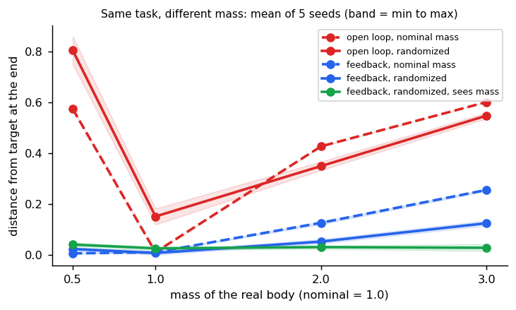
| Policy | Mass 0.5 | Mass 1.0 | Mass 2.0 | Mass 3.0 |
|---|---|---|---|---|
| Open loop, nominal mass | 0.574 | 0.010 | 0.427 | 0.601 |
| Open loop, randomized | 0.805 ± 0.039 | 0.151 ± 0.023 | 0.349 ± 0.012 | 0.548 ± 0.008 |
| Feedback, nominal mass | 0.005 ± 0.001 | 0.010 ± 0.001 | 0.126 ± 0.004 | 0.255 ± 0.003 |
| Feedback, randomized | 0.023 ± 0.006 | 0.007 ± 0.006 | 0.052 ± 0.007 | 0.124 ± 0.008 |
| Feedback, randomized, sees mass | 0.040 ± 0.010 | 0.025 ± 0.004 | 0.030 ± 0.005 | 0.027 ± 0.010 |
Mean and standard deviation over 5 seeds (the seed sets each policy's initialisation and the masses
drawn in training; the nominal open-loop policy has no randomness, so its spread is zero).
uv run --group tutorial python -m libs.tutorial.sim_to_real reproduces the table.
Three lessons, all visible in the table:
- A policy tuned to one simulator can be perfect there (0.010) and fail elsewhere (0.6).
- Randomization helps a policy that can react (feedback: error at mass 3 falls from 0.255 to 0.124) but cannot help one that cannot: the open-loop sequence just hedges, and is worse at the nominal mass (0.151 against 0.010).
- Giving the policy the information it needs (here the mass, as RMA's adaptation module infers it) beats hoping randomization averages it out: the worst error across the four masses is 0.040.
How wide should randomization be?
Randomization is a dial. Too narrow and the real world falls outside the training range; too wide and
the policy spends its capacity hedging against worlds that will never occur. The same feedback
policy, without seeing the mass, trained with five ranges (3 seeds; uv run --group tutorial python scripts/tutorial_results.py sim_to_real_more):
| Mass range in training | Error at mass 0.5 | at 1.0 | at 2.0 | at 3.0 |
|---|---|---|---|---|
| Nominal only (1.0) | 0.01 | 0.01 | 0.13 | 0.26 |
| 0.8 to 1.25 | 0.00 | 0.01 | 0.12 | 0.25 |
| 0.5 to 2.0 | 0.01 | 0.01 | 0.09 | 0.19 |
| 0.5 to 3.0 | 0.02 | 0.00 | 0.06 | 0.13 |
| 0.3 to 5.0 | 0.03 | 0.02 | 0.03 | 0.09 |
Read down the right-hand columns: each widening cuts the error at heavy masses (0.26 to 0.09) and costs a little at the light ones (0.01 to 0.03). Two practical rules follow. A range that barely exceeds the nominal value (0.8 to 1.25) changes almost nothing, so randomization has to be wide enough to cover real variation, including the cases you hope never happen. And you pay for width at the conditions you see most, so measure on the real distribution of conditions, not the worst case only. For driving, the analogue is the range of road friction, sensor mounting, latency and actor behaviour that the simulator samples.
Adaptation: infer the condition instead of hedging
The last row of the first table gives the policy the mass directly, which hardware cannot. RMA (2107.04034) shows how to get nearly the same thing without a mass sensor, in two phases, both in simulation:
- Train a teacher with privileged information. In simulation the mass is known, so the teacher policy sees it. This is the "feedback, randomized, sees mass" policy.
- Train an adaptation module to estimate it. It maps recent experience to the hidden condition, with the true condition as the label (free in simulation). On the robot, the module's estimate replaces the privileged input.
class AdaptationModule(nn.Module):
    """Infers the mass from recent experience: (v_t, v_t+1, force_t) -> mass.

    This is the idea of RMA's adaptation module. The teacher policy was trained seeing
    the true mass (privileged information); the student never sees it and instead
    estimates it from how its own forces changed its own velocity.
    """

    def __init__(self) -> None:
        """Creates a small MLP over one transition."""
        super().__init__()
        self.net = nn.Sequential(nn.Linear(3, 32), nn.Tanh(), nn.Linear(32, 1))

    def forward(self, transition: torch.Tensor) -> torch.Tensor:
        """Estimated mass per transition, shape (batch,)."""
        return self.net(transition).squeeze(-1)


def train_adaptation(
    teacher: nn.Module, steps: int = 1500, seed: int = 0
) -> AdaptationModule:
    """Fits the adaptation module on transitions generated by the teacher in simulation.

    The mass label comes for free in simulation, which is the whole trick: privileged
    information is available at training time and estimated at deployment.
    """
    torch.manual_seed(seed)
    module = AdaptationModule()
    optimizer = torch.optim.Adam(module.parameters(), lr=1e-2)
    for _ in range(steps):
        mass = 0.5 + 2.5 * torch.rand(64)
        x, v = torch.zeros(64), torch.zeros(64)
        batch, labels = [], []
        with torch.no_grad():
            for step in range(STEPS):
                force = teacher(torch.stack([x, v, mass], dim=-1), step).squeeze(-1)
                v_next = v + DT * (force - FRICTION * v) / mass
                batch.append(torch.stack([v, v_next, force], dim=-1))
                labels.append(mass)
                v, x = v_next, x + DT * v_next
        loss = ((module(torch.cat(batch)) - torch.cat(labels)) ** 2).mean()
        optimizer.zero_grad()
        loss.backward()
        optimizer.step()
    return module


@torch.no_grad()
def adapted_errors(teacher: nn.Module, module: AdaptationModule) -> dict[float, float]:
    """Final distance at each test mass when the policy gets an estimated mass.

    The estimate is the running mean of the module's output over the transitions seen
    so far in the episode (the first step has no history and uses the nominal 1.0).
    """
    errors = {}
    for mass in MASSES:
        m = torch.tensor([mass])
        x, v = torch.zeros(1), torch.zeros(1)
        estimates = []
        for step in range(STEPS):
            estimate = (
                torch.stack(estimates).mean(dim=0) if estimates else torch.ones(1)
            )
            force = teacher(torch.stack([x, v, estimate], dim=-1), step).squeeze(-1)
            v_next = v + DT * (force - FRICTION * v) / m
            estimates.append(module(torch.stack([v, v_next, force], dim=-1)))
            v, x = v_next, x + DT * v_next
        errors[mass] = (x - TARGET).abs().item()
    return errors
In the toy, the module reads one transition (the velocity before and after, and the force applied). A body at rest says little, so the estimate sharpens once it has moved: after 6 steps its errors for masses 0.7, 1.5 and 2.5 are within 0.35 (a test checks it). Across 3 seeds, with the running mean of the estimates feeding the teacher policy:
| Policy | Error at mass 0.5 | at 1.0 | at 2.0 | at 3.0 |
|---|---|---|---|---|
| Teacher, sees the true mass | 0.04 | 0.02 | 0.03 | 0.03 |
| Adapted from history | 0.03 | 0.02 | 0.03 | 0.08 |
| Blind, randomized 0.5 to 3.0 | 0.02 | 0.00 | 0.06 | 0.13 |
The adapted policy matches the teacher at three masses and is within 0.05 at the heaviest, where the estimates are noisiest and the first steps are spent with a wrong guess; it beats the blind policy at the heavy end (0.08 against 0.13). It is slightly worse than blind at the lightest mass, a reminder that estimation error is its own cost. In a real robot the "mass" is a vector of friction, payload, terrain and motor strength, and the module reads a window of recent states and actions.
Reference implementation (PyTorch)
Tests are in libs/tutorial/tests/test_sim_to_real.py; run uv run --group tutorial python -m libs.tutorial.sim_to_real.
def rollout(
    policy: nn.Module, mass: torch.Tensor, observe_mass: bool = False
) -> tuple[torch.Tensor, torch.Tensor]:
    """Simulates the point mass and returns the training cost and the final error.

    Args:
        policy: Called as ``policy(observation, step)``; returns a force (batch, 1).
        mass: Mass of each simulated body, shape (batch,).
        observe_mass: Whether the observation includes the mass.

    Returns:
        The cost per rollout (squared distance along the way, a control cost, and a
        heavy penalty for not being at the target and stopped at the end) and the
        absolute distance to the target at the end, each of shape (batch,).
    """
    x = torch.zeros_like(mass)
    v = torch.zeros_like(mass)
    cost = torch.zeros_like(mass)
    for step in range(STEPS):
        obs = [x, v] + ([mass] if observe_mass else [])
        force = policy(torch.stack(obs, dim=-1), step).squeeze(-1)
        v = v + DT * (force - FRICTION * v) / mass
        x = x + DT * v
        cost = cost + (x - TARGET) ** 2 + 0.01 * force**2
    cost = cost + 20 * (x - TARGET) ** 2 + 5 * v**2
return cost, (x - TARGET).abs()class OpenLoopPolicy(nn.Module):
"""A fixed sequence of forces, one per step, ignoring what it observes."""
def __init__(self) -> None:
"""Creates a zero force sequence."""
super().__init__()
self.force = nn.Parameter(torch.zeros(STEPS))
def forward(self, obs: torch.Tensor, step: int) -> torch.Tensor:
"""Returns the force for this step, repeated over the batch."""
return self.force[step].expand(len(obs), 1)
class FeedbackPolicy(nn.Module):
"""A small MLP from the observation to a force."""
def __init__(self, observe_mass: bool = False) -> None:
"""Creates the MLP; the input is (x, v) or (x, v, mass)."""
super().__init__()
inputs = 3 if observe_mass else 2
self.net = nn.Sequential(nn.Linear(inputs, 32), nn.Tanh(), nn.Linear(32, 1))
def forward(self, obs: torch.Tensor, step: int) -> torch.Tensor:
"""Returns the force for this observation (the step is not used)."""
return self.net(obs)def train_policy(
policy: nn.Module,
randomize: bool,
observe_mass: bool = False,
steps: int = 600,
seed: int = 0,
mass_range: tuple[float, float] = (0.5, 3.0),
) -> nn.Module:
"""Trains ``policy`` by gradient descent through the simulator.
Args:
policy: An ``OpenLoopPolicy`` or ``FeedbackPolicy``.
randomize: If True each batch draws masses from ``mass_range``; otherwise
every rollout uses the nominal mass 1.0.
observe_mass: Whether the policy's observation includes the mass.
steps: Number of optimisation steps.
seed: Random seed for the mass draws.
mass_range: Low and high mass for randomization.
"""
torch.manual_seed(seed)
low, high = mass_range
rate = 3e-2 if isinstance(policy, OpenLoopPolicy) else 1e-2
optimizer = torch.optim.Adam(policy.parameters(), lr=rate)
for _ in range(steps):
mass = low + (high - low) * torch.rand(64) if randomize else torch.ones(64)
loss = rollout(policy, mass, observe_mass)[0].mean()
optimizer.zero_grad()
loss.backward()
optimizer.step()
return policyCheck yourself
- Why can randomization make a policy worse at the nominal conditions?
- Why did randomization not help the open-loop policy?
- What does RMA's adaptation module add that randomization alone does not?
- Give two checks to do before blaming the reality gap on missing randomization.
- In the toy, what did widening the mass range from 0.8–1.25 to 0.3–5.0 gain and cost?
- What is privileged information in RMA, and why can the teacher use it but the deployed robot cannot?
- Name three quantities a driving simulator should randomize, and one way to check the range is wide enough.
Quiz
Answer each question; feedback appears as soon as you choose.
Sources
- Tobin et al., Domain Randomization, 2017.
- Rudin et al., Learning to Walk in Minutes, 2021.
- Makoviychuk et al., Isaac Gym, 2021.
- Kumar et al., RMA, 2021.
- Hwangbo et al., Learning agile and dynamic motor skills for legged robots, 2019.
- OpenAI et al., Learning Dexterous In-Hand Manipulation, 2018.
- Zhao et al., Sim-to-Real Transfer in Deep Reinforcement Learning for Robotics: a Survey, 2020.
Reinforcement learning for policies and reasoning
Policy gradients in depth: the advantage and GAE bias-variance dial, PPO's clip and KL penalty (three estimators compared), GRPO's group baseline and its subtle shrinkage, reward design in Alpamayo-R1, and reward hacking.
Preference learning and offline RL
Learning from human preferences without a reward model (DPO and the reward it implies, and why a chosen response can lose probability), and learning policies from a fixed dataset of logs (offline RL: extrapolation error, conservatism and in-sample methods, with a toy).