Diffusion

Idea

Destroy data with noise in small steps, then learn to undo each step. If you can reverse the destruction, you can start from pure noise and walk back to a sample of the data.

Two facts make this practical. Adding noise is trivial and needs no learning, so we can create as many (clean, noisy) training pairs as we like. And each step the network has to learn is small and local: given a slightly noisy sample, say which direction looks more like data, rather than producing a whole image from nothing. Chain a hundred or a thousand of those small corrections and you have a generator. This page builds the method in the order you would implement it. Calvin Luo's Understanding Diffusion Models: A Unified Perspective and Lilian Weng's What are diffusion models? cover the same ground in more depth.

Forward process (fixed, no learning)

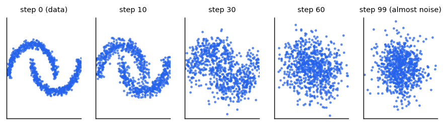
Take a data point x0. Over T steps add a little Gaussian noise each step until only noise remains. A useful property: you can jump straight to any step t in one shot,

$x_t = \sqrt{\bar\alpha_t}\, x_0 + \sqrt{1-\bar\alpha_t}\, \epsilon, \qquad \epsilon \sim \mathcal{N}(0, I)$

where $\bar\alpha_t$ falls from near 1 (little noise) to near 0 (all noise) as t grows.

For intuition with numbers: if $\bar\alpha_t = 0.5$, then $x_t = 0.71\,x_0 + 0.71\,\epsilon$, an equal mix of signal and noise.

The noise schedule

How fast $\bar\alpha_t$ falls is the noise schedule. Our toy uses 100 steps with a per-step noise amount $\beta_t$ rising linearly from 0.001 to 0.06, and $\bar\alpha_t$ is the running product of $(1-\beta_s)$:

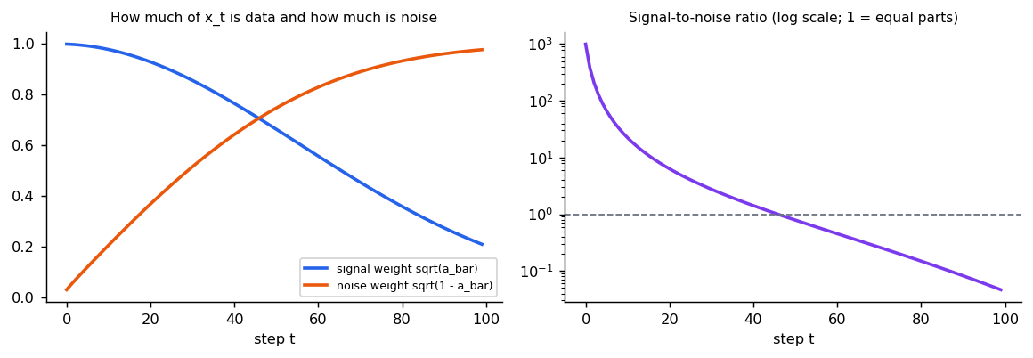
One property is worth knowing, and it is tested in our code: if the data has unit variance, then $x_t$ also has unit variance at every step, because $\bar\alpha_t \cdot 1 + (1-\bar\alpha_t) = 1$. The noising only trades signal for noise; it never blows up the scale. That keeps the network's inputs in a stable range.

class NoiseSchedule:
    """A linear beta schedule and the quantities derived from it."""

    def __init__(
        self, steps: int = 100, beta_start: float = 1e-3, beta_end: float = 0.06
    ):
        """Precomputes beta_t, alpha_t and the cumulative product alpha_bar_t."""
        self.steps = steps
        self.betas = torch.linspace(beta_start, beta_end, steps)
        self.alphas = 1.0 - self.betas
        self.alpha_bars = torch.cumprod(self.alphas, dim=0)

    def noisy(
        self, x0: torch.Tensor, t: torch.Tensor, noise: torch.Tensor
    ) -> torch.Tensor:
        """Jumps straight to step t: sqrt(alpha_bar) x0 + sqrt(1 - alpha_bar) noise."""
        bar = self.alpha_bars[t][:, None]
        return bar.sqrt() * x0 + (1 - bar).sqrt() * noise

Training (very simple)

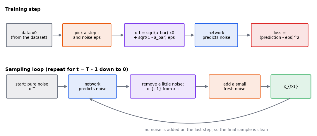
1. Sample a data point x0, a random step t, and noise eps.
2. Build x_t with the formula above.
3. Train a network to predict the noise: $\mathcal{L} = \lVert \epsilon - \epsilon_\theta(x_t, t)\rVert^2$.

That is the whole objective in the standard formulation. The network is given the noisy input and the step, and it is a regression problem, which is why training is stable compared with GANs.

class Denoiser(nn.Module):
    """Predicts the noise that was added, given the noisy point and the step."""

    def __init__(self, dim: int = 2, hidden: int = 128) -> None:
        """Creates a small MLP that takes (x_t, t / steps)."""
        super().__init__()
        self.net = nn.Sequential(
            nn.Linear(dim + 1, hidden),
            nn.SiLU(),
            nn.Linear(hidden, hidden),
            nn.SiLU(),
            nn.Linear(hidden, dim),
        )

    def forward(self, x_t: torch.Tensor, t_fraction: torch.Tensor) -> torch.Tensor:
        """Returns the predicted noise, same shape as ``x_t``."""
        return self.net(torch.cat([x_t, t_fraction[:, None]], dim=-1))


def diffusion_loss(
    model: Denoiser, schedule: NoiseSchedule, x0: torch.Tensor
) -> torch.Tensor:
    """Samples a step and noise per point and regresses the noise."""
    t = torch.randint(0, schedule.steps, (len(x0),))
    noise = torch.randn_like(x0)
    predicted = model(schedule.noisy(x0, t, noise), t / schedule.steps)
    return ((predicted - noise) ** 2).mean()

Why predict the noise?

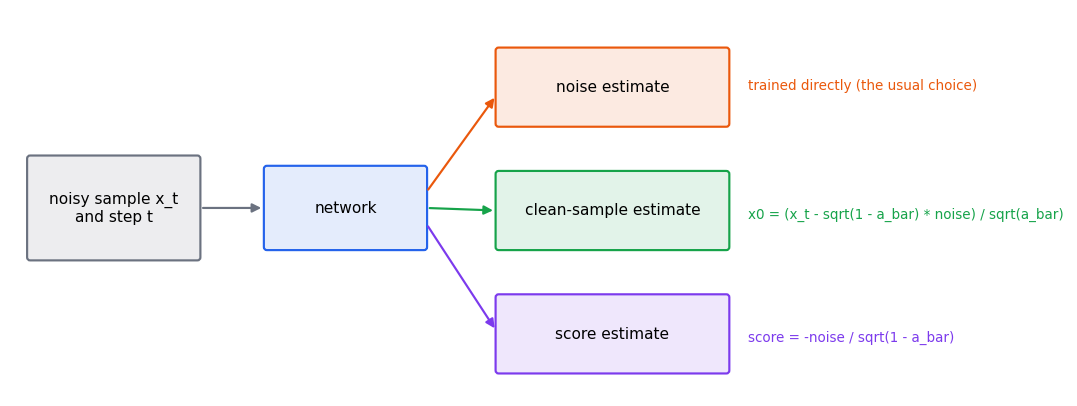
It can look odd to ask the network for the noise rather than the clean sample. They are the same information: given $x_t$ and the true noise, the clean sample follows by rearranging the formula,

$\hat x_0 = \frac{x_t - \sqrt{1-\bar\alpha_t}\,\hat\epsilon}{\sqrt{\bar\alpha_t}}, \qquad \text{score} = \nabla_{x_t} \log p(x_t) \approx -\frac{\hat\epsilon}{\sqrt{1-\bar\alpha_t}}$

So a network that predicts noise also gives a clean-sample estimate and the score, the direction in which the density of noisy data increases. Three views of one quantity; the noise form is the most common choice because its target has the same scale (unit variance) at every step. Song et al.'s score-based SDE paper develops the score view, and Yang Song's blog post is a gentle introduction.

def predict_x0(
    schedule: NoiseSchedule, x_t: torch.Tensor, t: torch.Tensor, noise: torch.Tensor
) -> torch.Tensor:
    """Recovers the clean sample implied by a noise estimate.

    Rearranging x_t = sqrt(bar) x0 + sqrt(1 - bar) noise gives
    x0 = (x_t - sqrt(1 - bar) noise) / sqrt(bar). Predicting the noise, the clean
    sample and the score are three views of the same quantity.
    """
    bar = schedule.alpha_bars[t][:, None]
    return (x_t - (1 - bar).sqrt() * noise) / bar.sqrt()


def score_from_noise(
    schedule: NoiseSchedule, t: torch.Tensor, noise: torch.Tensor
) -> torch.Tensor:
    """The score of x_t (gradient of its log density) is minus noise over its scale."""
    bar = schedule.alpha_bars[t][:, None]
    return -noise / (1 - bar).sqrt()


def gaussian_noise_predictor(
    schedule: NoiseSchedule, mean: float, std: float
) -> Callable[[torch.Tensor, torch.Tensor], torch.Tensor]:
    """The exact optimal noise predictor for one-dimensional data from N(mean, std^2).

    Then x_t is Gaussian with mean sqrt(bar) * mean and variance bar * std^2 + 1 - bar,
    and the best guess of the noise given x_t is a straight-line function of x_t. It
    lets us test the sampler without training anything.
    """

    def predict(x_t: torch.Tensor, t_fraction: torch.Tensor) -> torch.Tensor:
        t = (t_fraction * schedule.steps).round().long()
        bar = schedule.alpha_bars[t][:, None]
        variance = bar * std**2 + 1 - bar
        return (1 - bar).sqrt() * (x_t - bar.sqrt() * mean) / variance

    return predict


@torch.no_grad()
def loss_by_step(
    model: Denoiser, schedule: NoiseSchedule, x0: torch.Tensor, repeats: int = 20
) -> torch.Tensor:
    """Mean squared noise-prediction error at each step t, shape (steps,)."""
    errors = torch.zeros(schedule.steps)
    for t in range(schedule.steps):
        steps = torch.full((len(x0),), t)
        for _ in range(repeats):
            noise = torch.randn_like(x0)
            predicted = model(schedule.noisy(x0, steps, noise), steps / schedule.steps)
            errors[t] += ((predicted - noise) ** 2).mean().item() / repeats
    return errors

What the loss looks like

Is every step equally hard? No. We computed the trained toy denoiser's error at each step:

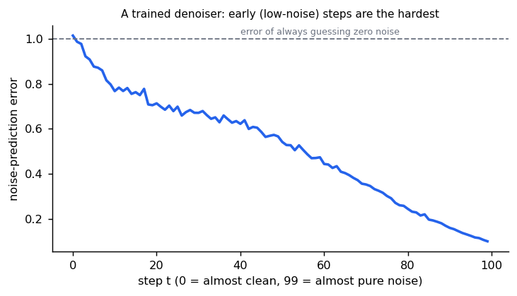
Over 3 seeds the error was 1.02 ± 0.03 at step 0, 0.55 ± 0.01 at step 50 and 0.10 ± 0.01 at step 99 (uv run --group tutorial python scripts/tutorial_results.py diffusion). The low-noise steps are the hardest to learn precisely, and later work such as the design-space paper below revisits how training steps are weighted and sampled.

Sampling

Start from x_T ~ N(0, I). For t from T down to 1, use the network's noise estimate to compute a slightly cleaner x_{t-1}. In the DDPM sampler each update is

$x_{t-1} = \frac{1}{\sqrt{\alpha_t}}\Big(x_t - \frac{\beta_t}{\sqrt{1-\bar\alpha_t}}\,\hat\epsilon_\theta(x_t, t)\Big) + \sqrt{\beta_t}\, z, \qquad z \sim \mathcal{N}(0, I)$

The first part subtracts a scaled noise estimate, which moves toward the data. The fresh noise $z$ (dropped on the last step) keeps the process a proper random walk, so different starting noise gives different samples; the DDIM sampler in the Sampling, guidance and diffusion policy module uses a different, deterministic update with no fresh noise and needs far fewer steps. The original method needs hundreds to thousands of steps. Later samplers reduce this a lot, but sampling stays iterative, which is the main cost.

NoisePredictor = Callable[[torch.Tensor, torch.Tensor], torch.Tensor]


@torch.no_grad()
def sample(
    predict_noise: NoisePredictor, schedule: NoiseSchedule, n: int, dim: int = 2
) -> torch.Tensor:
    """Starts from pure noise and removes the predicted noise step by step.

    Args:
        predict_noise: Called as ``predict_noise(x_t, t / steps)``; a trained
            ``Denoiser`` or any exact formula with that signature.
        schedule: The noise schedule.
        n: Number of samples.
        dim: Dimension of the data.
    """
    x = torch.randn(n, dim)
    for t in range(schedule.steps - 1, -1, -1):
        beta, alpha, bar = schedule.betas[t], schedule.alphas[t], schedule.alpha_bars[t]
        predicted = predict_noise(x, torch.full((n,), t / schedule.steps))
        x = (x - beta / (1 - bar).sqrt() * predicted) / alpha.sqrt()
        if t > 0:
            x = x + beta.sqrt() * torch.randn_like(x)
    return x

Testing the sampler without training anything

A sampler bug is easy to mistake for a training problem. So test the loop with a denoiser we can write down. If the data is one-dimensional $\mathcal{N}(\mu, \sigma^2)$, then $x_t$ is Gaussian with mean $\sqrt{\bar\alpha_t}\,\mu$ and variance $\bar\alpha_t\sigma^2 + 1 - \bar\alpha_t$, and the best noise estimate given $x_t$ is a straight line in $x_t$ (gaussian_noise_predictor in the code above). Sampling with it should reproduce $\mathcal{N}(\mu, \sigma^2)$:

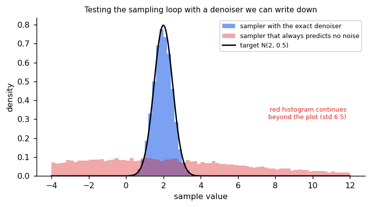
The tests check both outcomes: the exact denoiser recovers the mean within 0.06 and the standard deviation within 0.03, and the zero-noise predictor fails by a wide margin. Flipping the sign of the update or dropping the noise scale in the clean-sample formula makes the matching test fail.

Why it matters for actions

• Multimodal outputs. If the same scene has two valid actions (pass left or right), a regression network averages them into a bad middle action. A diffusion model represents the whole distribution and samples one mode.
• Conditioning. Feed the image, state or language as extra input to the network, so it generates actions given the observation. Classifier-free guidance trains with the condition sometimes dropped, then mixes both predictions at sampling to follow the condition more strongly (the Sampling, guidance and diffusion policy module).
• Score view. The noise estimate is also a score estimate, as above, which is why diffusion and score-based models are the same family.

On the toy two-moons data, the trained 100-step sampler put generated points 0.11 ± 0.01 from the nearest real point on average (3 seeds), about the data's own spread.

Where to go next

• Karras et al., Elucidating the Design Space of Diffusion-Based Generative Models, organises diffusion models into a design space and proposes improvements to sampling, training and score-network preconditioning.
• Compressing the data first, then diffusing in the latent space (the Discrete tokenizers and VAE modules), is how large image models make each step cheaper.
• Flow matching trains a closely related model with straighter paths that needs fewer steps.

Cost

Each denoising step is a network forward pass. A robot policy at 10 Hz cannot afford hundreds of steps, so robot and driving models use few steps, truncated schedules or flow matching (next module). DiffusionDrive, for example, reports getting diverse driving trajectories in 2 denoising steps by starting from anchored noise.

Reference implementation (PyTorch)

The code embedded above covers the noise schedule (including the one-shot jump to step t), the denoiser with its loss, the sampling loop, and the conversions and checks. Tests are in libs/tutorial/tests/test_diffusion.py; run uv run --group tutorial python -m libs.tutorial.diffusion.

Check yourself

1. Why does predicting noise make training a plain regression?
2. Why does an MSE-trained policy fail when two actions are equally good, and how does diffusion avoid it?
3. What is the trade-off in the number of sampling steps?
4. What does classifier-free guidance change at sampling time?
5. If you know the true noise in $x_t$, how do you get the clean sample back?
6. Why is the noise-prediction error close to 1 at the smallest noise levels?
7. What is the fresh noise in the sampling update for, and what happens if you remove it?
8. How can you test a sampler without training a network?

Quiz

Answer each question; feedback appears as soon as you choose.

Sources

• Ho et al., Denoising Diffusion Probabilistic Models, 2020.
• Song et al., Score-Based Generative Modeling through Stochastic Differential Equations, 2020.
• Nichol and Dhariwal, Improved Denoising Diffusion Probabilistic Models, 2021.
• Luo, Understanding Diffusion Models: A Unified Perspective, 2022.
• Karras et al., Elucidating the Design Space of Diffusion-Based Generative Models, 2022.
• Ho and Salimans, Classifier-Free Diffusion Guidance, 2022.
• Chi et al., Diffusion Policy, 2023.
• Liao et al., DiffusionDrive, 2024.