Driving data and labels
Common driving datasets and benchmarks, how labels are produced and checked, and how Alpamayo-R1 builds its reasoning labels.
Sources and confidence
Dataset sizes and sensor lists come from each dataset's paper abstract or, for the Physical AI dataset, its Hugging Face card. The Alpamayo-R1 labeling details were checked against the text of the paper's PDF (arXiv v2). Licences differ by dataset and often restrict use; read each one before downloading. Numbers here are not a ranking.
What a driving sample is
A training sample pairs sensor history (cameras, maybe lidar and radar, plus the car's motion) with a target. The target depends on the task:
| Task | Target | Where the label comes from |
|---|---|---|
| 3D detection and tracking | Boxes with class and track id | Human annotation, often assisted by models |
| Online mapping | Lane and boundary geometry | Human-built HD maps or annotation |
| Motion forecasting | Other agents' future paths | Free: later frames of the same log |
| Planning and imitation | The ego car's future trajectory | Free: what the human driver actually did |
| Question answering | Text answers about the scene | Humans, or a language model |
| Reasoning | Text explaining why an action is right | Humans, a language model, or both |
The useful fact for a robotics reader: for planning and forecasting, logs label themselves. The hard, expensive labels are the semantic ones: boxes, maps, language.
Common datasets
All entries are as the cited paper or card reports.
| Dataset | Sensors and scale | Typical use |
|---|---|---|
| nuScenes (2019) | 6 cameras, 5 radars, 1 lidar, all 360 degrees; 1000 scenes of 20 s; 3D boxes for 23 classes | Detection, tracking, open-loop planning; widely used baseline |
| Waymo Open (2019) | Camera and lidar; 1150 scenes of 20 s | Perception at larger scale and diversity |
| Waymo Open Motion (2021) | Over 100,000 scenes of 20 s at 10 Hz, more than 570 hours, mined for interactions | Interactive motion forecasting |
| Argoverse 2 (2023) | Three datasets: 1,000 annotated sensor sequences, 20,000 unlabeled lidar sequences, 250,000 mined forecasting scenarios | Perception, self-supervised lidar, forecasting |
| nuPlan (2021) | 1500 hours of human driving from four cities | Planning benchmark with a lightweight closed-loop simulator |
| BDD100K (2018) | 100K driving videos, 10 tasks | Diverse multitask vision |
| Physical AI Autonomous Vehicles (NVIDIA, 25.10) | 306,152 clips of 20 s, about 1,700 hours, 7 cameras on every clip, lidar on 298,326 clips, radar on up to 10 per clip for 160,761 clips; 25 countries, 2,500+ cities | Training and evaluating driving models, including the Alpamayo line |
Notes on the Physical AI card: the obstacle and ego-motion labels are machine-generated, not ground truth; a separate human-verified reasoning set covers a curated subset of out-of-distribution scenarios (1,450 train clips and 290 validation clips, test held out); access is gated, and its licence limits use to internal AV development and expires 12 months after download. That is a different footing from an academic dataset, so check it before building on it.
Benchmarks and simulators (evaluation data)
A model can match a logged trajectory and still drive badly (the Imitation learning module). Evaluation data comes in three kinds:
- Open loop on logs: compare the prediction with the recorded path (nuScenes style). Cheap, and the weakest evidence.
- Non-reactive simulation on real data: NAVSIM unrolls bird's-eye-view abstractions of real test scenes for a short horizon and computes simulation metrics such as progress and time to collision. Its paper positions it as a middle ground between open-loop and full closed-loop evaluation.
- Closed loop in simulation: CARLA is an open-source urban driving simulator. Bench2Drive is a multi-ability closed-loop benchmark built on it, which the authors motivate by the weakness of open-loop metrics. nuPlan (above) and AlpaSim, used by Alpamayo-R1, fill the same role.
Labeling strategies
Real pipelines mix four ingredients.
- Human annotation. Highest quality, highest cost. Typical for boxes and maps.
- Model-assisted or fully automatic labeling. A model proposes labels, humans check a sample. Cheap and scalable, but the dataset inherits the model's mistakes.
- Language-model labeling. A VLM or LLM writes question-answer pairs or explanations from the video and the known trajectory.
- Free labels from logs. Future motion of the ego car and of other agents.
The design question is always: which labels need humans, and how do you know the automatic ones are good enough? The usual answers are to have humans label or verify a fraction, to measure agreement between automatic and human labels, and to make the label format structured so errors are detectable.
Case study: Alpamayo-R1's Chain of Causation labels
What the paper describes (the CoC dataset has 700K video segments, drawn from 80,000 hours of driving in more than 2,500 cities in 25 countries):
- Structured taxonomy. Each clip gets at most one longitudinal and one lateral driving decision from a fixed list (for example set-speed tracking, lead-obstacle following, yield, stop for static constraints; lane change, merge or split, in-lane nudge, turn), or "None". Causal factors are open-ended: critical objects, traffic lights, stop or yield control, road events, lane lines, routing intent.
- Keyframes. Raw clips are 20 s long, and each training sample uses a 2 s history to predict a 6 s future. For reactive scenarios the keyframe sits about 0.5 s before the behaviour changes. Rule-based detectors label 10 Hz "meta actions" (accelerate, decelerate, steer), and transitions mark candidate keyframes.
- Leakage control. The labeler is shown only the 2 s of history when it identifies critical components, and the future only when it picks the decision, so it cannot explain the decision using the result.
- Two label sources. Human annotators work in two stages with a labeling tool that separates history from future, and a second annotator checks each label, with a sample sent to expert auditors. A model such as GPT-5 labels at scale offline, from video sampled at 2 Hz plus the ego trajectory and meta actions. The paper says the human-verified share is on the order of 10 percent, used for supervised fine-tuning, for evaluating the auto-labels, and for model evaluation.
- Checking the checker. GPT-5 acts as an evaluator of label quality on a curated 2K-sample set, and its judgments align with human evaluation 92 percent of the time. Structured labels improve a causal-relation score by 132.8 percent over free-form traces.
- Other training data. The backbone is pretrained on 3.7M VQA samples (24.7K driving video VQA), and the paper describes 100K further AV samples with critical-object annotations and next-action reasoning. The CoC data is used for supervised fine-tuning and for RL. For RL, the paper says scaling to the full pre-training data would be prohibitive in time and compute, so it selects samples where the model's output distribution disagrees most with a reward-based target, and mixes in a similar proportion of random samples to keep the data diverse. The size of the RL set is not stated.
Exercise: is the automatic labeler good enough?
Raw agreement can mislead when one class dominates. Cohen's kappa corrects for the agreement two labellers would reach by chance. Chance agreement is computed from how often each labeller uses each label: if both say "set-speed" 60 percent of the time, they agree on it 36 percent of the time even with their eyes closed. Kappa is the share of the remaining room that they actually fill:
where is observed agreement and is chance agreement. One means perfect agreement, zero means no better than chance. With a confusion matrix of human labels (rows) against automatic labels (columns) for three decisions, illustrative counts, not from any dataset:
def cohen_kappa(confusion: torch.Tensor) -> tuple[float, float, float]:
    """Raw agreement, chance agreement and Cohen's kappa from a confusion matrix.

    Rows are one labeller (say, human), columns the other (automatic). Chance
    agreement is what two labellers with these label frequencies, labelling
    independently, would agree on anyway.

    Raises:
        ValueError: If the matrix is not square.
    """
    if confusion.ndim != 2 or confusion.shape[0] != confusion.shape[1]:
        raise ValueError(f"need a square matrix, got shape {tuple(confusion.shape)}")
    confusion = confusion.double()
    total = confusion.sum()
    observed = confusion.trace() / total
    expected = (confusion.sum(0) * confusion.sum(1)).sum() / total**2
    return (
        observed.item(),
        expected.item(),
        ((observed - expected) / (1 - expected)).item(),
    )


def kappa_from_labels(a: torch.Tensor, b: torch.Tensor, classes: int) -> float:
    """Cohen's kappa for two label vectors."""
    confusion = torch.zeros(classes, classes)
    for x, y in zip(a.tolist(), b.tolist(), strict=True):
        confusion[x, y] += 1
    return cohen_kappa(confusion)[2]


def bootstrap_kappa(
    a: torch.Tensor, b: torch.Tensor, classes: int, resamples: int = 500, seed: int = 0
) -> tuple[float, float]:
    """A 95 percent bootstrap interval for kappa: resample the labelled items."""
    generator = torch.Generator().manual_seed(seed)
    values = []
    for _ in range(resamples):
        index = torch.randint(0, len(a), (len(a),), generator=generator)
        values.append(kappa_from_labels(a[index], b[index], classes))
    values.sort()
    return values[int(0.025 * resamples)], values[int(0.975 * resamples)]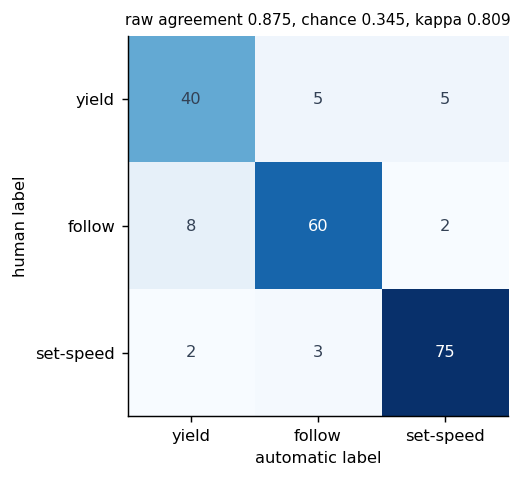
For the matrix above, raw agreement is 0.875, chance agreement 0.345 and kappa 0.809. Now a dominated
case: 1,000 clips where 94 percent are "no event", and the automatic labeler almost never flags the
rare class correctly ([[920, 20], [40, 20]]). Raw agreement is still 0.94, but chance agreement is
0.905 and kappa is 0.37. A labeler can look excellent by the raw number and be close to useless on
the cases you care about. For a rare class, also read per-class precision and recall off the matrix.
How certain is the kappa?
Kappa from 50 doubly-labelled clips is a noisy estimate. Resample the labelled items with replacement and recompute kappa to get an interval:
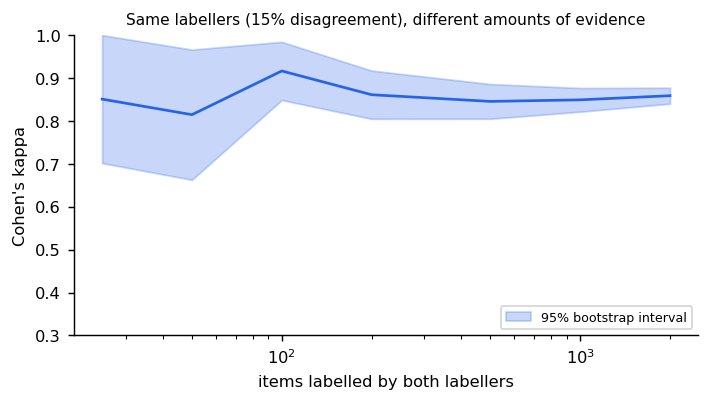
With the same labellers, the interval is about 0.67 to 0.94 at 50 items and 0.82 to 0.88 at 1,000. Before you reject a labeler (or accept one) on a kappa from a small sample, look at the interval.
How many labels does an audit need?
The question "what fraction of the automatic labels are wrong?" is estimating a proportion. For an error rate and a margin at 95 percent confidence, the number of items to check is roughly
def audit_sample_size(error_rate: float, margin: float, z: float = 1.96) -> int:
    """Items a human must check to estimate an error rate within +- ``margin``.

    Uses the normal approximation n = z^2 p (1 - p) / margin^2 (z = 1.96 for 95 percent
    confidence). The worst case is p = 0.5.

    Raises:
        ValueError: If ``error_rate`` is not in (0, 1) or ``margin`` is not positive.
    """
    if not 0 < error_rate < 1 or margin <= 0:
        raise ValueError(
            f"need 0 < error_rate < 1 and margin > 0, got {error_rate}, {margin}"
        )
    return math.ceil(z**2 * error_rate * (1 - error_rate) / margin**2)
If you expect 10 percent errors and want to know the rate within plus or minus 2 points, check 865 items. With no idea of the rate (the worst case, ) it is 2,401. Halving the margin to 1 point quadruples the sample to 3,458. The sample size does not depend on how big the dataset is, which is why a few thousand human-checked labels can audit millions of automatic ones, provided the sample is random. A sample picked because it was "interesting" estimates nothing about the rest.
Rule-based meta-actions and keyframes
Alpamayo-R1's keyframes come from rule-based detectors on the ego log. A minimal version labels each time step by its acceleration, then takes the frame a little before each change:
ACCELERATE, CRUISE, DECELERATE = 0, 1, 2


def meta_actions(
    speed: torch.Tensor, dt: float = 0.1, threshold: float = 0.5
) -> torch.Tensor:
    """Rule-based longitudinal labels from a speed log: accelerate, cruise, decelerate.

    The acceleration is the finite difference of speed; beyond +- ``threshold`` m/s^2
    it is labelled accelerate or decelerate.
    """
    accel = torch.diff(speed, prepend=speed[:1]) / dt
    labels = torch.full(speed.shape, CRUISE)
    labels[accel > threshold] = ACCELERATE
    labels[accel < -threshold] = DECELERATE
    return labels


def keyframes(labels: torch.Tensor, lead: int = 5) -> torch.Tensor:
    """Candidate keyframes: ``lead`` steps before each change of meta action.

    Taking the frame just before the behaviour changes gives the labeller a view of the
    situation that caused it, without yet showing the result.
    """
    changes = (labels[1:] != labels[:-1]).nonzero().squeeze(-1) + 1
    return (changes - lead).clamp(min=0)
For a car cruising and then braking, the label flips from cruise to decelerate at one step, and the keyframe (a lead of 5 steps, 0.5 s at 10 Hz) lands 5 steps before the flip. The labeller sees the situation that caused the braking without yet seeing the braking. Rules like these are cheap, deterministic and auditable, which is why they pick where to label and the expensive model or human decides what to write.
Mining the long tail
Training on raw logs teaches mostly "keep going". To find the rare scenes, score each scene by how far it sits from its neighbours in an embedding space (a pretrained perception model, say) and keep the highest scores:
def rarity_scores(embeddings: torch.Tensor, k: int = 10) -> torch.Tensor:
    """Mean distance to the k nearest other scenes; large means few look like it."""
    distances = torch.cdist(embeddings, embeddings)
    distances.fill_diagonal_(float("inf"))
    return distances.topk(k, largest=False).values.mean(dim=1)


def mining_study(
    k: int = 50, n: int = 5000, rare_share: float = 0.02, seed: int = 0
) -> tuple[float, float]:
    """Share of rare scenes in the top 5 percent by rarity score, and the base rate.

    Common scenes are one broad cluster; rare scenes are five tight clusters of
    ``n * rare_share / 5`` scenes each (a cut-in, an emergency vehicle, an odd one).
    A scene in a cluster of 20 has 19 close neighbours, so a score based on the
    ``k`` nearest neighbours only sees it as unusual if ``k`` exceeds the cluster size.
    """
    generator = torch.Generator().manual_seed(seed)
    rare = int(n * rare_share)
    common = torch.randn(n - rare, 8, generator=generator)
    centres = 4.0 * torch.randn(5, 8, generator=generator)
    which = torch.randint(0, 5, (rare,), generator=generator)
    unusual = centres[which] + 0.5 * torch.randn(rare, 8, generator=generator)
    embeddings = torch.cat([common, unusual])
    is_rare = torch.cat([torch.zeros(n - rare), torch.ones(rare)]).bool()
    top = rarity_scores(embeddings, k).topk(int(0.05 * n)).indices
    return is_rare[top].float().mean().item(), is_rare.float().mean().item()
The detail that matters is . A rare event such as a cut-in is not one odd scene but a small cluster of similar odd scenes. In the study above there are 5,000 scenes, 2 percent of them rare in five clusters of 20. A scene in a cluster of 20 has 19 close neighbours, so a score based on the 10 nearest neighbours calls it ordinary.
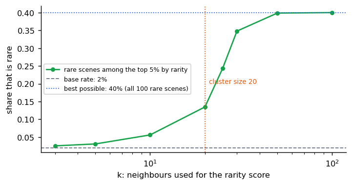
In our run, the top 5 percent by rarity were 5 percent rare at , 24 percent at and 40 percent at , which is every rare scene (100 rare scenes fill 40 percent of 250 slots). Choose larger than the clusters you want to find, check what comes out by looking at it, and do not assume that "far from everything" and "rare but real" are the same thing: sensor glitches are far from everything too.
Issues to keep in mind
- The long tail. Most driving is uneventful. Datasets either mine for interesting scenes (Waymo Open Motion, Argoverse 2 forecasting, Alpamayo's scenario-based clip selection) or oversample rare cases; training on raw logs teaches mostly "keep going". See the mining study above for how the choice of decides whether mining finds anything.
- Label noise from models. A model trained on model-made labels may learn the labeler's habits; measure it against a human-verified set.
- Leakage. If a label was written knowing the outcome, the model can learn to rely on text that would not exist at drive time.
- Open-loop trust. Strong open-loop numbers on logs do not establish safe driving (the Imitation learning module).
- Licences and privacy. Check redistribution, commercial use, expiry and personal-data limits before using a dataset.
Check yourself
- Which driving labels are free from logs, and which are expensive?
- Why is raw agreement a poor measure of label quality when one class dominates?
- How does showing the labeler only the history, then the future, reduce leakage?
- What does NAVSIM give that open-loop L2 error does not, and what does it still not give?
- What limits would you check on the Physical AI dataset before using it in a product?
- Why does the number of items you must audit not grow with the size of the dataset?
- A kappa of 0.8 comes from 40 doubly-labelled clips. What do you still need before trusting it?
Answers
- Free from logs: the ego car's future trajectory (the planning label), its speed and controls, and other agents' motion once a tracker has run. Expensive: 3D boxes, HD maps, driving decisions and reasoning text, which need people or a labelling model.
- When one class dominates, two labellers agree often by chance alone. In the example, raw agreement was 0.94 while kappa, which subtracts chance agreement, was 0.37: the labeller was nearly useless on the rare class that matters.
- At drive time the model only has the history. A labeller who has seen the outcome tends to explain the decision with it. Showing the history first means the causes are written from what was observable; the future is shown only to choose the decision.
- NAVSIM unrolls a bird's-eye-view abstraction of real test scenes for a short horizon and scores collisions, drivable area, progress and comfort, so a plan is judged by what it would do, not only by its distance to the log. It does not give long-horizon closed loop, agents that react, or re-rendered sensor input.
- The licence (commercial use, redistribution, expiry), personal-data and privacy limits, and the dataset card's own caveats, such as obstacle and ego-motion labels being machine-generated rather than ground truth.
- The sample size depends on the error rate and the margin you want (n = 1.96² p(1 − p) / margin²), not on how many items there are, provided the sample is random.
- An interval: with 50 items the bootstrap interval in the module was about 0.67 to 0.94, so 40 clips cannot rule out a mediocre labeller. Label more items at random, report the interval, and check per-class recall for the rare classes.
Quiz
Answer each question; feedback appears as soon as you choose.
Sources
Every dataset and benchmark above is linked inline; titles, identifiers and the dataset-card figures were checked at the time of writing. The Alpamayo-R1 labeling section is from arXiv 2511.00088.
State estimation and tracking
How a Kalman filter turns noisy detections into position and velocity, how to tell whether its noise settings are honest, what happens when measurements are missing, and where learned models replace it.
Planning and vehicle models
What a driving trajectory has to satisfy, the bicycle model, the Intelligent Driver Model, trajectory vocabularies, and why a simple rule-based planner is the baseline to beat.