Discrete tokenizers: VQ-VAE and FSQ
How continuous images and actions become a vocabulary of tokens: vector quantization and its training tricks, dead codes and how to measure and fix them, finite scalar quantization, and action tokenizers from per-step bins to FAST-style frequency coding.
Why discrete tokens
Language models predict one token from a fixed vocabulary at a time. Images, video and robot actions are continuous. To use the same machinery (the Transformers module) on them, a tokenizer has to turn each continuous signal into integers and back. The VAE module's encoder and decoder are the starting point; the new part is a quantizer in the middle that forces the latent onto a finite set of values.
What a tokenizer has to balance
| Property | Why it matters | Measured by |
|---|---|---|
| Fidelity | Decoding the tokens should give back the signal | Reconstruction error |
| Length | Every token is a step for the transformer (attention cost, latency) | Tokens per image or per action chunk |
| Vocabulary use | Unused tokens waste capacity | Code usage and perplexity |
| Bits per token | for codes | 8 bits for 256 codes, 10 for 1,024 |
A tokenizer is a compression scheme, and the three numbers trade against each other: a 16 by 16 grid of tokens from a 1,024-code vocabulary carries bits per image, whatever the image's resolution, which is why the decoder has to be good at filling in detail.
Vector quantization (VQ-VAE)
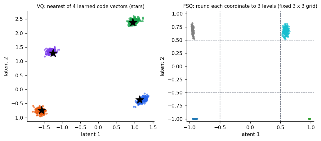
Neural Discrete Representation Learning (1711.00937) introduced the VQ-VAE. Keep a learned codebook of K vectors. The encoder output is replaced by its nearest codebook vector, and the index of that vector is the token. Two practical details:
- Straight-through gradient. Picking the nearest entry is not differentiable. The trick copies the decoder's gradient straight back to the encoder output as if quantization were the identity.
- Two extra loss terms. One moves codebook entries toward the encoder outputs, and the commitment term keeps the encoder from drifting away from its chosen entry.
Dead codes
Because the codebook is learned, some entries can end up never chosen, so those tokens are wasted and clusters of data are squashed onto another cluster's code. This is called codebook collapse. In the exercise below, the same four-cluster task with four codes failed in 5 of 20 runs that differed only in their random initialisation (a run counts as failed if its final reconstruction error exceeds 0.2).
Measuring and fixing dead codes
Two numbers tell you whether a codebook is healthy: the share of codes that are used at all, and the perplexity of their frequencies, , which reads as the effective vocabulary size (equal to when every code is used equally, 1 when one code takes everything). Log both during training.
@torch.no_grad()
def restart_dead_codes(
    quantizer: VectorQuantizer, z: torch.Tensor, dead: torch.Tensor
) -> int:
    """Moves each dead code onto a random encoder output; returns how many moved.

    A code nobody chooses gets no gradient and never recovers on its own. Placing it
    where the data actually is gives it a chance to win some inputs back.
    """
    count = int(dead.sum())
    if count:
        picks = torch.randint(0, len(z), (count,))
        quantizer.codebook.weight[dead] = z[picks]
    return count


def codebook_usage(indices: torch.Tensor, num_codes: int) -> tuple[float, float]:
    """Share of codes used, and perplexity exp(entropy) of their frequencies.

    Perplexity equals ``num_codes`` when every code is used equally and 1 when one
    code takes everything: the effective vocabulary size.
    """
    counts = torch.bincount(indices, minlength=num_codes).float()
    probs = counts / counts.sum()
    nonzero = probs[probs > 0]
    entropy = -(nonzero * nonzero.log()).sum()
    return (counts > 0).float().mean().item(), entropy.exp().item()
In the toy, healthy runs use all 4 codes with perplexity 4.0; a collapsed run uses 3 of 4 (perplexity 2.8) and its reconstruction error is 2.1 instead of 0.02, because two clusters share one code. Common remedies:
- Restart dead codes: every so often, move any code that was not chosen onto a random recent
encoder output. In the toy this cut failed runs from 5 of 20 to 2 of 20 (
restart=True). - Initialise from the data: set the codebook to k-means centres of early encoder outputs.
- Update codes by moving averages (EMA) instead of gradients, which tends to keep them closer to the data.
- Avoid the codebook altogether: FSQ, below.
Finite scalar quantization (FSQ)
Finite Scalar Quantization: VQ-VAE Made Simple (2309.15505) proposes replacing the codebook with something much simpler: project the latent down to a few dimensions, and round each dimension to a small set of fixed values. The implicit codebook is the product of those sets (levels [3, 3] gives 9 codes; [5, 5, 5, 5] gives 625). As the abstract notes, the same downstream models trained on VQ-VAE tokens can be trained on these.
With no learned codebook there is nothing to go dead. In our exercise FSQ with levels [3, 3] failed in 0 of 20 runs, on the same seeds as VQ above. That is a toy result, not a claim about large models; the FSQ paper reports its own comparisons.
Tokenizing actions
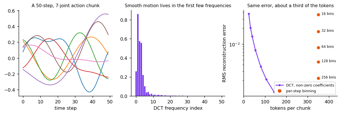
Actions need a tokenizer too if a language model is to output them as tokens (the VLA models module). Two designs, and the trade-off between them, are easy to measure on a smooth 50-step chunk of 7 joint commands:
def bin_tokens(
    chunk: torch.Tensor, bins: int, low: float = -1.0, high: float = 1.0
) -> tuple[torch.Tensor, torch.Tensor]:
    """Per-step, per-dimension binning (as in RT-2 and OpenVLA): one token per number.

    Returns:
        Integer tokens with the chunk's shape, and the de-tokenised chunk (bin
        centres).
    """
    width = (high - low) / bins
    tokens = ((chunk.clamp(low, high - 1e-6) - low) / width).floor().long()
    return tokens, low + (tokens.float() + 0.5) * width


def dct_matrix(n: int) -> torch.Tensor:
    """Orthonormal DCT-II matrix: row k is the k-th cosine basis over n samples."""
    k = torch.arange(n)[:, None].float()
    i = torch.arange(n)[None, :].float()
    matrix = torch.cos(torch.pi / n * (i + 0.5) * k) * (2.0 / n) ** 0.5
    matrix[0] /= 2**0.5
    return matrix


def dct_tokens(chunk: torch.Tensor, scale: float) -> tuple[torch.Tensor, torch.Tensor]:
    """FAST-style tokens: DCT along time, scale, round to integers.

    Smooth motion puts almost all its energy in the low-frequency coefficients, so
    after rounding most high-frequency coefficients are 0. FAST then compresses the
    integer sequence further with byte-pair encoding; here we just count non-zeros.

    Args:
        chunk: Actions, shape (time, dims).
        scale: Multiplier before rounding; larger keeps more detail and more tokens.

    Returns:
        The integer coefficients (time, dims) and the reconstructed chunk.
    """
    basis = dct_matrix(chunk.shape[0])
    coefficients = (basis @ chunk * scale).round()
    return coefficients.long(), basis.T @ (coefficients / scale)


def smooth_chunk(steps: int = 50, dims: int = 7, seed: int = 0) -> torch.Tensor:
    """A smooth multi-joint action chunk: a few low-frequency sines per dimension."""
    generator = torch.Generator().manual_seed(seed)
    t = torch.linspace(0, 1, steps)[:, None]
    freqs = torch.rand(3, dims, generator=generator) * 2 + 0.2
    phases = torch.rand(3, dims, generator=generator) * 6.28
    amps = torch.rand(3, dims, generator=generator) * 0.3
    return (
        amps[None] * torch.sin(6.28 * freqs[None] * t[..., None] + phases[None])
    ).sum(1)
Per-step binning (RT-2, OpenVLA) cuts each joint's range into bins and emits one token per joint per time step: always tokens. More bins reduce the error (at most half a bin) but not the length.
Frequency coding (FAST, 2501.09747) first applies a discrete cosine transform along time, the transform JPEG uses for images. Smooth motion puts nearly all its energy in the first few frequencies, so after scaling and rounding most coefficients are zero; FAST then compresses the remaining integers further with byte-pair encoding (the Tokens, ViT and VLMs module).
| Tokenizer | Tokens for the chunk | RMS error |
|---|---|---|
| Binning, 64 bins | 350 | 0.0085 |
| Binning, 256 bins | 350 | 0.0022 |
| DCT, scale 20 | 55 non-zero | 0.0077 |
| DCT, scale 100 | 106 non-zero | 0.0021 |
The DCT reaches 256-bin accuracy with about a third of the tokens, before any byte-pair encoding. The gain depends on smoothness: jerky, high-frequency motion has energy at every frequency and compresses less. The FAST paper reports that per-step binning performs poorly on dexterous, high-frequency data, which is where its method helps most.
Reference implementation (PyTorch)
Tests are in libs/tutorial/tests/test_quantization.py and include the straight-through gradient,
the nearest-code property, the grid bounds, usage and perplexity, dead-code restarts (which reduce
failed runs), binning's half-bin error bound, and the DCT's orthonormality and compression. Run
uv run --group tutorial python -m libs.tutorial.quantization.
class VectorQuantizer(nn.Module):
    """Snaps each vector to its nearest entry in a learned codebook."""

    def __init__(self, num_codes: int, dim: int, beta: float = 0.25) -> None:
        """Creates the codebook.

        Args:
            num_codes: Number of codebook entries (the vocabulary size).
            dim: Size of each entry.
            beta: Weight of the commitment loss that keeps the encoder near its code.
        """
        super().__init__()
        self.num_codes = num_codes
        self.codebook = nn.Embedding(num_codes, dim)
        self.codebook.weight.data.uniform_(-1.0, 1.0)
        self.beta = beta

    def forward(
        self, z: torch.Tensor
    ) -> tuple[torch.Tensor, torch.Tensor, torch.Tensor]:
        """Quantizes ``z`` of shape (batch, dim).

        Returns:
            The quantized vectors (with a straight-through gradient to ``z``), the
            integer code indices (batch,), and the VQ loss.
        """
        indices = torch.cdist(z, self.codebook.weight).argmin(dim=-1)
        chosen = self.codebook(indices)
        # Move codebook entries toward the encoder outputs, and the encoder toward
        # its chosen entries (the commitment term).
        loss = ((chosen - z.detach()) ** 2).mean()
        loss = loss + self.beta * ((z - chosen.detach()) ** 2).mean()
        # Straight-through estimator: the forward pass uses the code, the backward
        # pass pretends quantization was the identity.
return z + (chosen - z).detach(), indices, lossclass FiniteScalarQuantizer(nn.Module):
"""Rounds each dimension to a few fixed levels; no codebook is learned."""
def __init__(self, levels: list[int]) -> None:
"""Creates the quantizer.
Args:
levels: Number of levels per dimension; every entry must be odd. The
vocabulary size is the product of the levels.
Raises:
ValueError: If any level count is even or smaller than 3.
"""
super().__init__()
if any(level < 3 or level % 2 == 0 for level in levels):
raise ValueError(f"levels must be odd and at least 3, got {levels}")
self.register_buffer("levels", torch.tensor(levels))
@property
def num_codes(self) -> int:
"""Size of the implicit codebook."""
return int(self.levels.prod().item())
def forward(self, z: torch.Tensor) -> tuple[torch.Tensor, torch.Tensor]:
"""Quantizes ``z`` of shape (batch, len(levels)).
Returns:
Quantized values in [-1, 1] (straight-through gradient) and one integer
code per row in [0, num_codes).
"""
half = (self.levels - 1) / 2
bounded = torch.tanh(z) * half
rounded = bounded + (bounded.round() - bounded).detach()
digits = (rounded + half).long()
radix = torch.cumprod(
torch.cat([torch.ones(1, dtype=torch.long), self.levels[:-1]]), dim=0
)
return rounded / half, (digits * radix).sum(dim=-1)def failed_runs(
make_quantizer: Callable[[], nn.Module],
seeds: range,
steps: int = 1200,
threshold: float = 0.2,
*,
restart: bool = False,
) -> int:
"""Counts training runs whose final reconstruction error exceeds ``threshold``.
A bad run usually means a codebook entry was never used (a "dead code"), so a
whole cluster is reconstructed as another one. The quantizer is created after
seeding, so a seed fixes its initialisation too.
"""
failures = 0
for seed in seeds:
torch.manual_seed(100 + seed)
_, _, _, error = train_autoencoder(
make_quantizer(), steps, seed, restart=restart
)
failures += int(error > threshold)
return failuresWhere this appears
- Image generation. VQGAN (2012.09841) and latent diffusion (2112.10752) both generate in a compressed latent space of an autoencoder instead of in pixels.
- Actions. Discrete action tokens in a VLA (see the VLA models module) are a tokenizer problem; FAST compresses the action sequence before tokenising it.
- Driving. AutoVLA (2506.13757) tokenizes continuous trajectories into discrete, feasible actions so one autoregressive model can generate them.
Check yourself
- Why does a VQ-VAE need a straight-through estimator?
- What is a dead code, and why does it hurt?
- How many codes does FSQ with levels [5, 3] have, and which parameters does it learn?
- Give one reason to prefer a continuous action expert over discrete tokens (see the VLA module).
- A codebook of 512 codes has perplexity 40. What does that tell you, and what would you try?
- Why does a DCT need fewer tokens than per-step binning for a smooth chunk, and when would it not?
Answers
- Choosing the nearest codebook entry has no useful gradient. The straight-through estimator copies the decoder's gradient back to the encoder output as if quantization were the identity, so the encoder can still learn.
- A codebook entry that is never chosen. Its token is wasted capacity, and the data it should have covered is squashed onto another code: in the toy a collapsed run reconstructs with error 2.1 instead of 0.02.
- 5 × 3 = 15 codes. It learns no codebook at all: only the projections before and after the rounding.
- Discrete tokens are generated one at a time and limited by quantisation; a continuous expert produces a whole smooth chunk in a few steps and handles several good answers (the VLA module's action-head comparison).
- Only about 40 codes are effectively used: most of the codebook is dead or rarely used. Try restarting dead codes, initialising from k-means, EMA updates, or switching to FSQ.
- Smooth motion puts nearly all its energy in a few low frequencies, so most DCT coefficients round to zero. Jerky, high-frequency motion has energy everywhere and compresses much less.
Quiz
Answer each question; feedback appears as soon as you choose.
Sources
- Van den Oord et al., Neural Discrete Representation Learning, 2017.
- Mentzer et al., Finite Scalar Quantization, 2023.
- Esser et al., Taming Transformers for High-Resolution Image Synthesis, 2020.
- Rombach et al., High-Resolution Image Synthesis with Latent Diffusion Models, 2021.
Variational autoencoders
From autoencoders to VAEs: the latent-variable view, the ELBO, the closed-form KL, the reparameterisation trick, the beta trade-off and posterior collapse, with runnable code.
Diffusion
Denoising diffusion models explained step by step: the noise schedule, why predicting noise works, the loss, sampling, and three equivalent views, with figures and code you can check.