Scaling laws and data recipes
How loss falls with data, model size and compute, how to size a model for a budget, and the data work that decides results: de-duplication, mixtures, and mining the long tail.
Why this module
Foundation-model teams spend most of their effort on data, not architecture. Waymo's Staff "Foundation Models Recipes" role, for example, owns the pre- and post-training data recipe: filtering, de-duplication, long-tail mining, scaling ladders and data-mix optimisation. This module covers the two ideas behind that work: scaling laws, which say how much better a model gets with more data, parameters or compute, and data recipes, which decide what the data is.
For engineers from modular stacks this is familiar ground under new names: disengagement triage and scenario coverage become long-tail mining, and regression suites become evaluation sets per scenario category (From modular stacks to end-to-end).
1. Scaling laws
Kaplan et al. (2001.08361) found that a language model's loss falls as a power law in model size, dataset size and training compute, over many orders of magnitude, and that larger models use data more efficiently. A power law with a floor looks like
where is data (or parameters, or compute), how fast the loss falls, and the part no amount of removes (noise in the labels, an under-sized model). On a log-log plot the first term is a straight line, which is what makes extrapolation possible.
Reading a power law
Three habits make scaling plots easy to read:
- Think in factors, not increments. With , every doubling of data multiplies the reducible error by : about 19 percent less, whether you go from 100 to 200 scenes or from 100 million to 200 million. Each further gain costs twice as much data as the last.
- Watch the floor. Near the curve flattens and the straight-line fit stops working. If the floor is high, more of the same data will not help; better labels, a larger model or a different input will.
- Distrust a single run. Seeds move the points (see the table below), so fit several and look at the spread before extrapolating.
def fit_power_law(
    sizes: list[float], losses: list[float]
) -> tuple[float, float, float]:
    """Fits loss = a * size^(-alpha) + floor.

    For each candidate floor below the smallest loss, log(loss - floor) is linear in
    log(size); the floor with the smallest squared error in log space wins.

    Returns:
        (a, alpha, floor).

    Raises:
        ValueError: If fewer than three points are given.
    """
    if len(sizes) < 3:
        raise ValueError(f"need at least 3 points, got {len(sizes)}")
    log_n = torch.tensor([math.log(s) for s in sizes])
    target = torch.tensor(losses)
    best = None
    for floor in torch.linspace(0.0, min(losses) * 0.999, 400):
        log_l = torch.log(target - floor)
        slope, intercept = _line(log_n, log_l)
        error = ((intercept + slope * log_n - log_l) ** 2).sum().item()
        if best is None or error < best[0]:
            best = (error, math.exp(intercept), -slope, floor.item())
    _, a, alpha, floor = best
    return a, alpha, floor


def _line(x: torch.Tensor, y: torch.Tensor) -> tuple[float, float]:
    x_mean, y_mean = x.mean(), y.mean()
    slope = ((x - x_mean) * (y - y_mean)).sum() / ((x - x_mean) ** 2).sum()
    return slope.item(), (y_mean - slope * x_mean).item()


def power_law(size: float, a: float, alpha: float, floor: float) -> float:
    """Evaluates a fitted power law."""
    return a * size ** (-alpha) + floor
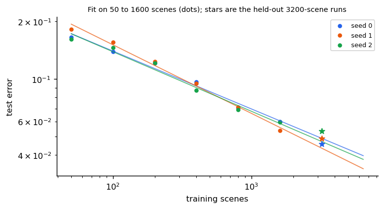
The toy: the end-to-end braking planner from the modular-to-end-to-end module, trained on 50 to 1,600 scenes. Fit a power law, then predict the error at 3,200 scenes before running it:
| Seed | Fitted exponent | Predicted error at 3,200 | Measured |
|---|---|---|---|
| 0 | 0.30 | 0.049 | 0.046 |
| 1 | 0.36 | 0.044 | 0.049 |
| 2 | 0.31 | 0.047 | 0.053 |
The prediction is within 0.006 of the measurement each time. That is the practical use of a scaling ladder: run a few cheap sizes, fit, and decide whether the expensive run is worth it before paying for it. It also shows the limits: three seeds give three different exponents, so a ladder needs repeats, and a fit says nothing beyond the range where the trend holds.
Robots and cars show similar trends. Lin et al. (2410.18647) report that imitation-learning policies generalise roughly as a power law in the number of training environments and objects, and that diversity of environments and objects matters more than the number of demonstrations. Alpamayo-R1 reports consistent improvements when scaling its model from 0.5 to 7 billion parameters.
2. Compute-optimal sizing
For a fixed compute budget , should you train a bigger model on less data or a smaller one on more? "Training Compute-Optimal Large Language Models" (Chinchilla, 2203.15556) found that large models of the time were undertrained, and that model size and training tokens should grow in equal proportion. Chinchilla (70B parameters, trained on about four times more data than the 280B Gopher) beat Gopher and reached 67.5 percent on MMLU.
A common rule of thumb read from that result is about 20 training tokens per parameter. With (the Training at scale module) and :
def compute_optimal(
    flops: float, tokens_per_param: float = 20.0
) -> tuple[float, float]:
    """Model size and data size for a compute budget, scaling both together.

    Uses C = 6 N D with D = k N, so N = sqrt(C / (6 k)). k of about 20 tokens per
    parameter is the usual reading of the Chinchilla result.

    Returns:
        (parameters, tokens).
    """
    params = math.sqrt(flops / (6.0 * tokens_per_param))
    return params, tokens_per_param * params
Chinchilla itself is the check: 70B parameters on 1.4 trillion tokens is about FLOPs, and the rule returns exactly that size and data for that budget.
Where the rule comes from
The paper estimates the optimum three ways. The third fits a formula to all its runs, with one term for the model's size and one for its data:
is the irreducible loss (the entropy of text), the second term is the cost of a finite model and the third the cost of finite data. Fix the budget and the two terms trade off: a bigger model leaves fewer tokens. Each budget has a best model size, which the paper derives in closed form:
# Hoffmann et al. (2022), approach 3: L(N, D) = E + A / N^alpha + B / D^beta, fitted on
# their language-model runs (N parameters, D training tokens).
CHINCHILLA = {"E": 1.69, "A": 406.4, "B": 410.7, "alpha": 0.34, "beta": 0.28}


def chinchilla_loss(params: float, tokens: float) -> float:
    """Predicted loss from the parametric fit: irreducible + model-size + data terms."""
    c = CHINCHILLA
    return c["E"] + c["A"] / params ** c["alpha"] + c["B"] / tokens ** c["beta"]


def optimal_allocation(flops: float) -> tuple[float, float]:
    """The (parameters, tokens) minimising the fitted loss subject to 6 N D = C.

    Closed form from the paper: N_opt = G (C / 6)^a with a = beta / (alpha + beta) and
    G = (alpha A / (beta B))^(1 / (alpha + beta)); D_opt = (C / 6) / N_opt.
    """
    c = CHINCHILLA
    g = (c["alpha"] * c["A"] / (c["beta"] * c["B"])) ** (1 / (c["alpha"] + c["beta"]))
    a = c["beta"] / (c["alpha"] + c["beta"])
    params = g * (flops / 6) ** a
    return params, flops / (6 * params)


def isoflop_curve(flops: float, sizes: list[float]) -> list[float]:
    """Fitted loss of each model size when the budget fixes the data at C / (6 N)."""
    return [chinchilla_loss(n, flops / (6 * n)) for n in sizes]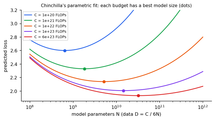
The fit agrees with the headline result (it predicts a lower loss for Chinchilla's 70B on 1.4T tokens than for Gopher's 280B on 300B tokens; a test checks this) but not with the exact ratio: at Chinchilla's budget this fit's optimum is about 32B parameters and 3 trillion tokens, around 90 tokens per parameter, and the paper itself notes that this approach projects a 40B optimum for Gopher's budget, smaller than its other two approaches. Its table for the first approach gives 20 billion tokens for a 1-billion-parameter model, the source of the "20 tokens per parameter" rule. The lesson: the direction (train smaller models on more data than was usual) is robust; the exact ratio depends on how you fit, and on your data.
Two cautions for driving: the 20-to-1 ratio was measured for language models, and a car's model is sized by the onboard latency budget at least as much as by training compute (Deploying a driving VLA); then the question becomes how much data a model of the deployable size can still use.
3. Data recipes
De-duplication
Repeating data adds no information. In the toy, 500 scenes each repeated 4 times give exactly the error of the 500 scenes alone (0.080 for seed 0; 0.079 and 0.085 for seeds 1 and 2), while 2,000 different scenes reach 0.057 to 0.060 with the same number of training rows:
def duplicate_run(unique: int, copies: int, seed: int = 0) -> float:
    """Test error when ``unique`` scenes are each repeated ``copies`` times.

    The training set has unique x copies rows and the same number of optimiser steps
    whatever the split, so this isolates what repetition is worth compared with new
    data.
    """
    base = scenes(unique, seed)
    train = {key: value.repeat_interleave(copies, dim=0) for key, value in base.items()}
    torch.manual_seed(seed)
    model = _fit(train, torch.ones(unique * copies))
    test = scenes(20000, 999)
    with torch.no_grad():
        correct = model(test["raw"]).argmax(dim=1) == test["brake"]
    return 1.0 - correct.float().mean().item()
(In this full-batch toy a repeated row changes nothing at all; with mini-batches repetition adds noise and overfitting risk, but still no information.) At scale it does harm as well. Lee et al. (2107.06499) found near-duplicates in common language datasets caused over 1 percent of model outputs to be verbatim copies of training text; de-duplicating cut memorised output tenfold and needed fewer training steps for the same accuracy. Driving logs have their own duplicates: hours of the same highway, the same depot loop, the same commute. Clustering scenes by embedding and capping each cluster is the driving equivalent.
Mixtures
Data comes from many sources (cities, sensors, weather, simulation, human demonstrations), and their proportions matter. DoReMi (2305.10429) tunes domain weights with a small 280M-parameter proxy model and reports that an 8B model trained on the reweighted mixture improves few-shot accuracy by 6.5 points and reaches the baseline's accuracy with 2.6 times fewer steps. The lesson that transfers: choose the mixture with small, cheap runs, the same way you choose the model size.
The long tail
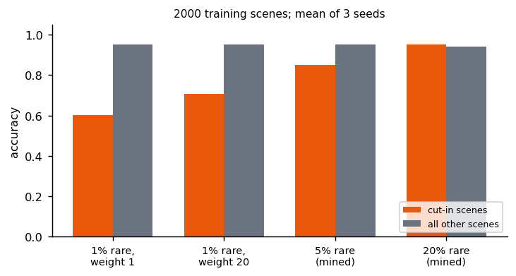
The scenes that matter most are rare: cut-ins, emergency vehicles, unusual road users. In the toy, cut-ins are only 1 percent of a 2,000-scene training set. Two responses: up-weight the rare scenes in the loss, or mine more real examples of them from the fleet.
def long_tail_dataset(
    size: int, rare_share: float, seed: int = 0
) -> dict[str, torch.Tensor]:
    """A training set in which cut-in scenes are only ``rare_share`` of the data."""
    pool = scenes(size * 20, seed)
    rare = pool["cut_in"].nonzero().squeeze(1)
    common = (~pool["cut_in"]).nonzero().squeeze(1)
    n_rare = max(1, round(size * rare_share))
    keep = torch.cat([rare[:n_rare], common[: size - n_rare]])
    return {key: value[keep] for key, value in pool.items()}


def long_tail_run(
    rare_weight: float, size: int = 2000, rare_share: float = 0.01, seed: int = 0
) -> dict[str, float]:
    """Trains with the rare scenes' loss multiplied by ``rare_weight``.

    Returns:
        Accuracy on cut-in scenes and on all other scenes of a balanced test pool.
    """
    train = long_tail_dataset(size, rare_share, seed)
    weights = torch.where(train["cut_in"], rare_weight, 1.0)
    torch.manual_seed(seed)
    model = _fit(train, weights)
    test = scenes(20000, 999)
    with torch.no_grad():
        correct = model(test["raw"]).argmax(dim=1) == test["brake"]
    return {
        "cut-in": correct[test["cut_in"]].float().mean().item(),
        "other": correct[~test["cut_in"]].float().mean().item(),
    }
| Training set (2,000 scenes) | Cut-in accuracy | Other scenes |
|---|---|---|
| 1 percent cut-ins | 0.60 ± 0.10 | 0.95 |
| 1 percent cut-ins, weighted 20 times | 0.71 ± 0.05 | 0.95 |
| 5 percent cut-ins (mined) | 0.85 ± 0.02 | 0.95 |
| 20 percent cut-ins (mined) | 0.95 ± 0.00 | 0.94 |
Up-weighting helps, but 20 examples weighted 20 times are still 20 examples: the model sees the same few cases louder. Mining 100 or 400 real ones teaches the variety. Over-representing the rare case costs a little on everything else (0.95 to 0.94 at 20 percent), which is the trade-off a mixture decides.
4. The data flywheel
Put together, a driving team's data loop looks like this:
- Trigger: find interesting scenes in fleet data, from disengagements, disagreements between the model and a teacher or rule (shadow mode), uncertainty, or a search over scene embeddings.
- Curate: de-duplicate, cluster, balance the mixture, keep evaluation sets per category.
- Label: human labels where needed, a large teacher model or offline auto-labelling where possible (Driving data and labels, Distillation).
- Train on a scaling ladder before a big run (Training at scale).
- Evaluate by scenario category, open and closed loop (Evaluating driving models), then deploy and repeat.
Owning this loop end to end, rather than one model in it, is what the Staff-level postings describe.
Reference implementation (PyTorch)
libs/tutorial/scaling_data.py; tests are in libs/tutorial/tests/test_scaling_data.py: the fit
recovers an exact power law; Chinchilla's own size and data come out of the compute-optimal rule;
the parametric fit's closed-form optimum matches a grid search, prefers Chinchilla to Gopher, and
favours more tokens per parameter as budgets grow; repeated scenes are worth no more than the unique
ones;
the toy error halves with data and the fit predicts the 3,200-scene error within 0.01; the long-tail
dataset has the requested share; and mining real examples beats up-weighting a few, which beats
doing nothing, with other scenes unaffected. Run uv run --group tutorial python -m libs.tutorial.scaling_data.
Check yourself
- What does a straight line on a log-log plot of loss against data mean, and what does the floor represent?
- Why does a scaling ladder need several seeds?
- Using and 20 tokens per parameter, what model size is compute-optimal for ?
- Why might a driving model not follow the compute-optimal size?
- Why did mining 100 cut-ins beat weighting 20 cut-ins 20 times?
- With , how much more data does it take to halve the reducible error?
- Why does the parametric fit disagree with the 20-tokens-per-parameter rule, and what survives the disagreement?
Quiz
Answer each question; feedback appears as soon as you choose.
Sources
- Kaplan et al., Scaling Laws for Neural Language Models, 2020.
- Hoffmann et al., Training Compute-Optimal Large Language Models, 2022 (Chinchilla).
- Lin et al., Data Scaling Laws in Imitation Learning for Robotic Manipulation, 2024.
- Lee et al., Deduplicating Training Data Makes Language Models Better, 2021.
- Xie et al., DoReMi, 2023.
- NVIDIA et al., Alpamayo-R1, 2025.
VLA models
How RT-2, OpenVLA, pi0 and SmolVLA turn a vision-language model into a robot policy: the anatomy of a forward pass, how actions come out (measured on an ambiguous instruction), training recipes, and how to diagnose a VLA that fails.
Co-training and catastrophic forgetting
Why fine-tuning a model on a new task erases the old one, a toy that measures it, and four ways to limit it: mixing old data back in, penalising important weights, small learning rates, and adapters.