Training at scale
How a large model is trained across many GPUs: where the memory goes, data, sharded, tensor and pipeline parallelism, the collectives they use, mixed precision and loss scaling, activation checkpointing, batch size and learning-rate schedules, and estimating cost and time.
Why this module
Every senior posting for driving and robot foundation models asks for experience training at scale: multi-node runs, large datasets, knowing the framework's internals. For a software engineer this is the most approachable gap, because most of it is systems work: memory budgets, communication, throughput and failure handling. It is also where a training run most often fails for reasons that have nothing to do with the model.
The page follows one question: how do you train a model that does not fit on one GPU, fast enough to matter? It builds the answer in layers:
- What one training step does, and where its memory goes (sections 1 and 2).
- Splitting the batch across GPUs, and the collective operations that keep the copies in sync (sections 3 and 4).
- Splitting the model itself: sharding, tensor and pipeline parallelism (sections 5 to 7).
- Making each GPU do more: mixed precision and activation checkpointing (sections 8 and 9).
- The optimisation side of scale: batch size, learning rate, stability (section 10).
- Estimating cost and checking efficiency (sections 11 and 12).
Every claim that can be checked numerically is checked in libs/tutorial/training_scale.py, on a
laptop, without GPUs.
1. One training step
A step has four phases, and every technique on this page changes one of them:
- Forward pass: run the batch through the model, keeping the intermediate results (activations) that the backward pass will need.
- Backward pass: compute the gradient of the loss with respect to every weight, layer by layer from the output back to the input, consuming the saved activations.
- Synchronise (only with several GPUs): combine the gradients computed on different GPUs.
- Optimiser step: update the weights from the gradients, using the optimiser's running state.
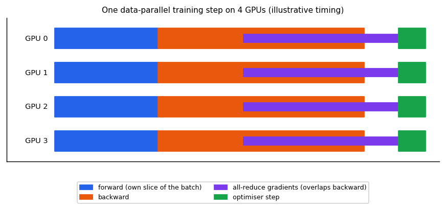
The backward pass costs about twice the forward pass: for every weight it computes two products, one for the gradient with respect to the layer's input (to keep going backwards) and one for the gradient with respect to the weight itself. That is where the "6" in the compute estimate of section 11 comes from: 2 operations per weight per token forward, 4 backward.
2. Where the memory goes
Training holds four things on the GPU: the weights, their gradients, the optimiser state and the activations. The first three depend only on the number of parameters. For the standard recipe, bf16 mixed precision with the Adam optimiser (1412.6980), they cost per parameter:
| Item | Bytes per parameter | Why it exists |
|---|---|---|
| bf16 weights | 2 | Used in the forward and backward passes |
| bf16 gradients | 2 | Output of the backward pass |
| fp32 master copy of the weights | 4 | Small updates would vanish in bf16 (section 8) |
| Adam first moment (fp32) | 4 | Running average of the gradient (momentum) |
| Adam second moment (fp32) | 4 | Running average of the squared gradient (per-weight step size) |
| Total model state | 16 |
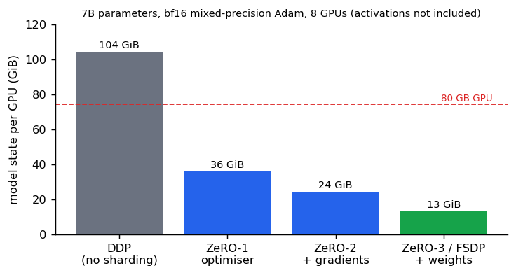
A 7-billion-parameter model therefore needs about 104 GiB of model state, more than one 80 GB GPU holds, before a single activation is stored. A 1B model needs about 15 GiB, which is why a 24 GB GPU such as an RTX 3090 can fully fine-tune models up to roughly a billion parameters if activations stay small, and needs LoRA or sharding beyond that (Efficient fine-tuning and inference).
def training_memory_gib(params: float, gpus: int = 1, zero_stage: int = 0) -> float:
    """Per-GPU memory for model state in bf16 mixed-precision Adam training.

    Per parameter: 2 bytes bf16 weights, 2 bytes bf16 gradients, and 12 bytes of
    fp32 optimiser state (master weights, Adam's first and second moments): 16 bytes.
    ZeRO shards across ``gpus``: stage 1 the optimiser state, stage 2 also the
    gradients, stage 3 (FSDP) also the weights. Activations are extra and not counted.

    Raises:
        ValueError: If ``zero_stage`` is not 0 to 3 or ``gpus`` is below 1.
    """
    if zero_stage not in (0, 1, 2, 3) or gpus < 1:
        raise ValueError(
            f"need zero_stage in 0..3 and gpus >= 1, got {zero_stage}, {gpus}"
        )
    weights, grads, optimiser = 2.0, 2.0, 12.0
    if zero_stage >= 1:
        optimiser /= gpus
    if zero_stage >= 2:
        grads /= gpus
    if zero_stage >= 3:
        weights /= gpus
    return params * (weights + grads + optimiser) / GIB


def training_flops(params: float, tokens: float) -> float:
    """Approximate training compute: 6 FLOPs per parameter per token.

    2 for the forward pass (a multiply and an add per weight) and 4 for the backward
    pass (gradients for activations and for weights).
    """
    return 6.0 * params * tokens


def training_days(
    params: float, tokens: float, gpus: int, peak_tflops: float, utilisation: float
) -> float:
    """Wall-clock days given GPU count, peak throughput and model FLOPs utilisation."""
    seconds = training_flops(params, tokens) / (gpus * peak_tflops * 1e12 * utilisation)
    return seconds / 86400
Activations
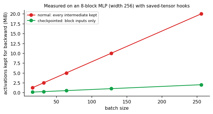
Activations are the other half, and often the bigger one. Every layer keeps its inputs, and often intermediate results, until the backward pass reaches it. The reference code counts exactly what autograd saves, using PyTorch's saved-tensor hooks, for an 8-block MLP of width 256:
def saved_activation_bytes(
    model: nn.Module, x: torch.Tensor, checkpointed: bool
) -> int:
    """Bytes of tensors autograd keeps from the forward pass for the backward pass.

    Uses ``saved_tensors_hooks`` to see every tensor saved for backward. With
    ``checkpointed``, each block of ``model`` (an ``nn.Sequential`` of blocks) runs
    under activation checkpointing, so only its input is kept and the rest is
    recomputed during the backward pass.
    """
    total = 0
    weights = {p.untyped_storage().data_ptr() for p in model.parameters()}

    def pack(tensor: torch.Tensor) -> torch.Tensor:
        nonlocal total
        if (
            tensor.untyped_storage().data_ptr() not in weights
        ):  # weights are not new memory
            total += tensor.numel() * tensor.element_size()
        return tensor

    with torch.autograd.graph.saved_tensors_hooks(pack, lambda tensor: tensor):
        hidden = x
        for block in model:
            if checkpointed:
                hidden = checkpoint(block, hidden, use_reentrant=False)
            else:
                hidden = block(hidden)
    return total


def deep_mlp(width: int = 256, blocks: int = 8, seed: int = 0) -> nn.Sequential:
    """A stack of residual-free MLP blocks, each Linear -> GELU -> Linear -> GELU."""
    torch.manual_seed(seed)
    return nn.Sequential(
        *(
            nn.Sequential(
                nn.Linear(width, 4 * width),
                nn.GELU(),
                nn.Linear(4 * width, width),
                nn.GELU(),
            )
            for _ in range(blocks)
        )
    )
Per block and per example it keeps the block's input (256 numbers), the hidden layer before and after the GELU (2 × 1024) and the output before the second GELU (256): 2,560 floats, about 10 KB. For 8 blocks and a batch of 64 that is 5 MiB, and doubling the batch doubles it; a test checks the exact byte count. The general rule: activation memory grows with batch × sequence length × width × depth, and attention adds a term that grows with the square of the sequence length unless an attention kernel such as FlashAttention avoids storing the score matrix. For a driving VLA with thousands of image tokens per sample, activations usually dominate model state.
3. Data parallelism: more GPUs, same model
The simplest way to use GPUs: put a full copy of the model on each, give each a different slice
of the batch, and average the gradients before the optimiser step. Every copy then takes the same
step and stays identical. PyTorch's DistributedDataParallel (DDP) does this.
It works because the gradient of an average loss is the average of the per-slice gradients. The reference code checks it: four replicas on quarter-batches, averaged, match one full batch to 1e-6.
def full_batch_gradient(x: torch.Tensor, y: torch.Tensor) -> list[torch.Tensor]:
    """Gradient of the mean squared error over the whole batch, on one device."""
    model = _model()
    ((model(x) - y) ** 2).mean().backward()
    return _grads(model)


def data_parallel_gradient(
    x: torch.Tensor, y: torch.Tensor, ranks: int
) -> list[torch.Tensor]:
    """Each rank holds a replica and a shard of the batch; gradients are averaged.

    This is what DistributedDataParallel's all-reduce does after the backward pass.
    """
    shards = zip(x.chunk(ranks), y.chunk(ranks), strict=True)
    per_rank = []
    for xs, ys in shards:
        replica = _model()
        ((replica(xs) - ys) ** 2).mean().backward()
        per_rank.append(_grads(replica))
    return [torch.stack(g).mean(dim=0) for g in zip(*per_rank, strict=True)]


def accumulated_gradient(
    x: torch.Tensor, y: torch.Tensor, micro_batches: int
) -> list[torch.Tensor]:
    """One replica, several backward passes before the optimiser step.

    Each micro-batch loss is divided by the number of micro-batches so the summed
    gradients equal the full-batch mean.
    """
    model = _model()
    for xs, ys in zip(x.chunk(micro_batches), y.chunk(micro_batches), strict=True):
        (((model(xs) - ys) ** 2).mean() / micro_batches).backward()
    return _grads(model)


def checkpointed_gradient(x: torch.Tensor, y: torch.Tensor) -> list[torch.Tensor]:
    """Activation checkpointing: drop the first block's activations, recompute later.

    Saves memory at the cost of a second forward pass through the block; the
    gradient is unchanged.
    """
    model = _model()
    first, rest = model[:2], model[2:]
    hidden = checkpoint(first, x, use_reentrant=False)
    ((rest(hidden) - y) ** 2).mean().backward()
    return _grads(model)
The same identity gives gradient accumulation: run several small batches through one GPU, add their gradients (each loss divided by the number of micro-batches), and step once. It reaches a large effective batch on few GPUs at the cost of time. Two things break the equivalence in practice: batch normalisation (its statistics are per replica, not per global batch) and anything tuned for a specific batch size, such as the learning rate (section 10).
Data parallelism alone does not reduce memory per GPU at all: every GPU still holds the full 16 bytes per parameter. It only adds throughput.
4. Collectives: how GPUs combine numbers
Distributed training is built from a few collective operations, each called on all GPUs at once:
| Collective | Before | After | Used for |
|---|---|---|---|
| All-reduce | Each GPU has a tensor | Each GPU has the sum (or mean) | Averaging gradients in DDP |
| Reduce-scatter | Each GPU has a tensor | Each GPU has the sum of one slice | Sharded gradients (ZeRO-2/3) |
| All-gather | Each GPU has one slice | Each GPU has the full tensor | Rebuilding sharded weights (ZeRO-3) |
| Broadcast | One GPU has a tensor | All GPUs have it | Initial weights |
An all-reduce is a reduce-scatter followed by an all-gather. The ring algorithm does it with bandwidth that does not depend on the number of GPUs: arrange the GPUs in a ring, cut each tensor into chunks, and pass chunks to the right neighbour.
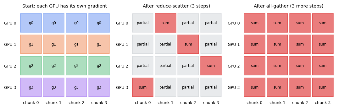
def ring_all_reduce(tensors: list[torch.Tensor]) -> tuple[list[torch.Tensor], int]:
    """Sums one tensor per rank with the ring algorithm; returns results and traffic.

    Each tensor is cut into N chunks. Reduce-scatter: in N - 1 steps every rank sends
    one chunk to its right neighbour, which adds it to its own; afterwards rank r holds
    the full sum of chunk (r + 1) mod N. All-gather: N - 1 more steps pass the finished
    chunks round the ring. Every rank sends 2 (N - 1) chunks, 2 (N - 1) / N of the
    tensor, however many ranks there are.

    Returns:
        The summed tensor on every rank, and the number of elements each rank sent.
    """
    n = len(tensors)
    chunks = [list(t.clone().chunk(n)) for t in tensors]
    sent = 0
    for step in range(n - 1):
        outgoing = [chunks[r][(r - step) % n].clone() for r in range(n)]
        for r in range(n):
            chunks[(r + 1) % n][(r - step) % n] += outgoing[r]
        sent += outgoing[0].numel()
    for step in range(n - 1):
        outgoing = [chunks[r][(r + 1 - step) % n].clone() for r in range(n)]
        for r in range(n):
            chunks[(r + 1) % n][(r + 1 - step) % n] = outgoing[r]
        sent += outgoing[0].numel()
    return [torch.cat(c) for c in chunks], sent


def tensor_parallel_mlp(
    x: torch.Tensor, w1: torch.Tensor, w2: torch.Tensor, shards: int
) -> torch.Tensor:
    """Megatron-style MLP across ``shards`` devices: one all-reduce, at the end.

    W1 is split by columns, so each device computes its own slice of the hidden layer
    and applies GELU to it without talking to the others. W2 is split by rows to
    match, so each device produces a partial output; summing the partials (the one
    all-reduce) gives exactly GELU(x W1) W2.
    """
    partials = [
        nn.functional.gelu(x @ w1_part) @ w2_part
        for w1_part, w2_part in zip(
            w1.chunk(shards, dim=1), w2.chunk(shards, dim=0), strict=True
        )
    ]
    return torch.stack(partials).sum(dim=0)


def pipeline_bubble(stages: int, micro_batches: int) -> float:
    """Idle share of a GPipe schedule with K stages and M micro-batches.

    Equals (K - 1) / (M + K - 1): each stage waits K - 1 slots for the pipeline to fill
    and K - 1 slots for it to drain, out of M + K - 1 per pass.
    """
    return (stages - 1) / (micro_batches + stages - 1)
Each GPU sends chunks of size , so about twice the tensor size, whatever is. A worked example with round, hypothetical numbers: a 7B model's bf16 gradients are 14 GB; each GPU sends about GB per step on 8 GPUs; at an effective 100 GB/s per GPU that is about 0.25 s. If the step's compute takes 1.7 s (section 11's example), the communication fits inside the backward pass, which is why frameworks start reducing the last layers' gradients while earlier layers are still computing (the overlap in the step figure).
5. Sharding: ZeRO and FSDP
Data parallelism stores the same optimiser state, gradients and weights on every GPU. ZeRO (Zero Redundancy Optimizer, 1910.02054) removes the copies by sharding: each GPU keeps only its slice and fetches the rest when needed.
| Stage | Sharded | Memory per parameter on 8 GPUs | Communication vs DDP |
|---|---|---|---|
| DDP | nothing | 16 bytes | 1× |
| ZeRO-1 | optimiser state | 2 + 2 + 12/8 = 5.5 bytes | 1× |
| ZeRO-2 | + gradients | 2 + 2/8 + 12/8 = 3.75 bytes | 1× |
| ZeRO-3 (FSDP) | + weights | 16/8 = 2 bytes | 1.5× |
The ZeRO paper states the communication column: partitioning optimiser state and gradients keeps the same communication volume as data parallelism, and partitioning the weights adds about 50 percent. It reports training models over 100 billion parameters on 400 GPUs. PyTorch's FSDP (Fully Sharded Data Parallel, 2304.11277) is the stage-3 design and reports performance comparable to DDP while supporting much larger models.
What FSDP does in one step, layer by layer:
- Forward: all-gather the layer's weight shards into a full layer, compute, free the gathered weights, keep the activations.
- Backward: all-gather the weights again, compute the gradients, reduce-scatter them so each GPU keeps only its slice of the summed gradient, free the weights.
- Optimiser step: each GPU updates only its own shard, with its own shard of the Adam state.
Only one or two layers are ever fully materialised, so memory per GPU scales down with . The cost is the extra all-gather in the backward pass, the 1.5×.
6. Tensor parallelism: splitting one layer
When even one layer is too large, or too slow, split the matrix multiplications themselves. Megatron-LM (1909.08053) splits a transformer's MLP so that it needs only one all-reduce in the forward pass: the first weight matrix by columns, so each GPU computes its own slice of the hidden layer and applies GELU to it independently, and the second by rows, so each GPU produces a partial output that one sum completes.
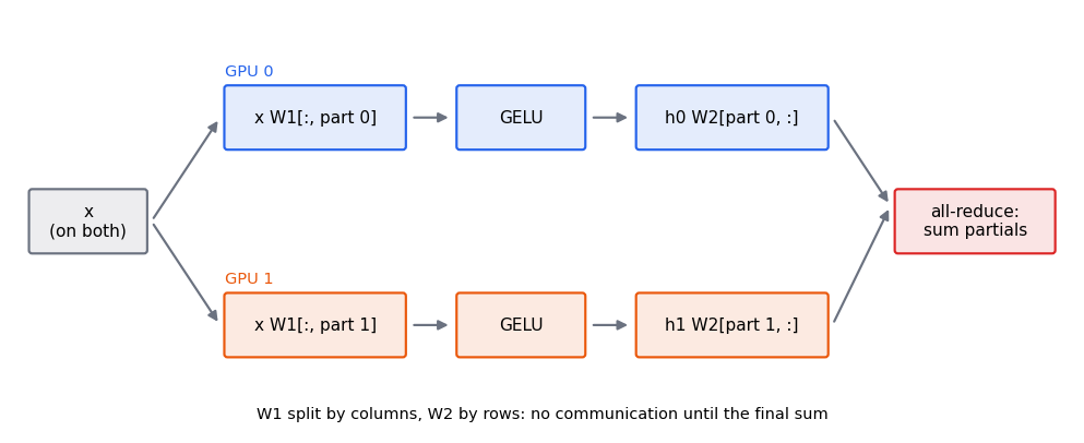
tensor_parallel_mlp in the collectives code above checks that the four-way split equals the unsplit layer. Attention splits the
same way, by heads. Megatron-LM reports training models up to 8.3 billion parameters on 512 GPUs with
76 percent scaling efficiency. Because tensor parallelism communicates inside every layer, it needs
the fastest links and usually stays within one machine.
7. Pipeline parallelism: splitting the depth
Pipeline parallelism puts consecutive groups of layers ("stages") on different GPUs and passes activations between them. Naively only one stage works at a time. GPipe (1811.06965) splits each batch into micro-batches so the stages work on different micro-batches at once. What remains idle, the bubble, is of the time for stages:
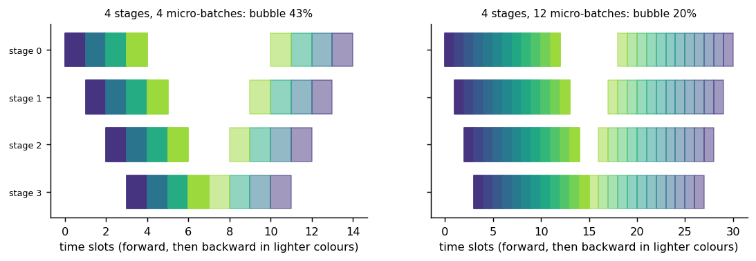
GPipe reports the bubble overhead to be negligible when . Large runs combine all three splits ("3D parallelism": data × tensor × pipeline); a run of a few billion parameters on one or two nodes usually needs only FSDP.
Choosing a strategy
| Situation | Usually enough |
|---|---|
| Model state fits on one GPU, want speed | DDP |
| Model state does not fit, a few nodes | FSDP (ZeRO-3), plus activation checkpointing |
| Single layers too large or slow | Add tensor parallelism inside each node |
| Hundreds of GPUs, very deep model | Add pipeline parallelism across nodes |
8. Mixed precision and loss scaling
Training in 16-bit halves memory and traffic and runs matrix multiplies much faster. The number formats differ in where they spend their bits:
| Format | Exponent bits | Mantissa bits (stored) | Largest value | Smallest positive (subnormal) |
|---|---|---|---|---|
| fp32 | 8 | 23 | about 3.4e38 | about 1.4e-45 |
| fp16 | 5 | 10 | 65504 | about 6e-8 () |
| bf16 | 8 | 7 | about 3.4e38 | about 9e-41 |
fp16 has precision but little range: small gradients underflow to zero. Mixed Precision Training (1710.03740) keeps fp32 master weights and multiplies the loss by a loss scale before the backward pass, which multiplies every gradient by the same factor and shifts them into range; the optimiser divides it back out in fp32. The paper notes that any value below becomes zero in fp16, and reports scale factors from 8 to 32K across its networks (many needed none).
FP16_SMALLEST = 2.0**-24  # smallest positive fp16 (subnormal) number, about 6e-8
FP16_LARGEST = 65504.0


def fp16_cast_losses(values: torch.Tensor, scale: float = 1.0) -> tuple[float, float]:
    """Shares of values lost when cast to fp16 after multiplying by ``scale``.

    Anything below 2^-24 in magnitude becomes zero (underflow); anything above 65504
    becomes infinite (overflow). Multiplying the loss by ``scale`` multiplies every
    gradient by it, which rescues small gradients; the optimiser divides by ``scale``
    again in fp32. Too large a scale overflows instead, which is why dynamic loss
    scaling lowers the scale whenever an infinity appears.

    Returns:
        (share that underflowed to zero, share that overflowed to infinity).
    """
    cast = (values * scale).to(torch.float16)
    return (cast == 0).float().mean().item(), cast.isinf().float().mean().item()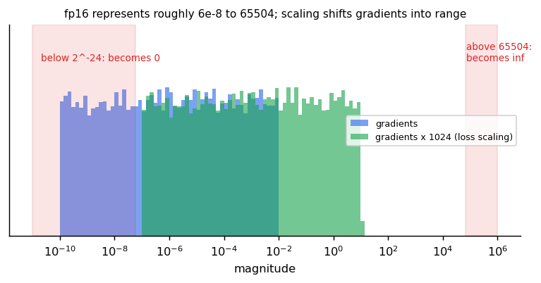
Too large a scale overflows to infinity, so frameworks use dynamic loss scaling: start high, halve the scale and skip the step whenever an infinity appears, and grow it slowly otherwise.
bf16 has fp32's range and much less precision, so it needs no loss scaling, which is why it is the default on recent GPUs and TPUs. Its weakness is the other one: with 7 stored mantissa bits, numbers near 1.0 are about apart, and a typical update is far smaller:
def accumulate_updates(
    dtype: torch.dtype, steps: int = 1000, update: float = 1e-4
) -> float:
    """Adds a small update to a weight of 1.0, ``steps`` times, stored in ``dtype``.

    bf16 stores 7 mantissa bits, so near 1.0 its spacing is 2^-7, about 0.0078; an
    update of 1e-4 rounds away to nothing every time. This is why mixed-precision
    training keeps an fp32 master copy of the weights for the optimiser step.
    """
    weight = torch.tensor(1.0, dtype=dtype)
    for _ in range(steps):
        weight = weight + torch.tensor(update, dtype=dtype)
return weight.float().item()| Weights stored in | Weight after 1000 updates of 1e-4, starting at 1.0 |
|---|---|
| bf16 | 1.0000 (every update rounded away) |
| fp32 | 1.1000 |
That is why the optimiser updates an fp32 master copy and casts it to bf16 for the next forward pass, and why section 2 counts 4 extra bytes per parameter.
9. Activation checkpointing
Activation checkpointing (also called rematerialisation) keeps only some activations in the forward pass and recomputes the rest in the backward pass, trading compute for memory. The gradient is unchanged (a test checks it to 1e-6). Checkpointing every block of the 8-block MLP keeps only each block's input:
Chen et al. (1604.06174) report cutting a 1,000-layer ResNet from 48 GB to 7 GB for about 30 percent more time. Recomputing everything is wasteful for large transformers; Korthikanti et al. (2205.05198) recompute only selected parts and add sequence parallelism, reporting 5 times less activation memory, over 90 percent less recomputation overhead, and 54.2 percent MFU training a 530B model on 2,240 A100 GPUs.
10. Batch size, learning rate and stability
Scale changes the optimisation, not only the systems:
- Bigger batches need a larger learning rate, introduced gradually. Goyal et al. (1706.02677) trained ResNet-50 with minibatches of 8,192 images on 256 GPUs in one hour without losing accuracy, using a linear scaling rule (multiply the learning rate by the batch-size factor) and a warmup that ramps the learning rate up over the first steps.
- Warmup then decay. A common schedule is a linear warmup and a cosine decay:
def learning_rate(
    step: int, peak: float, warmup: int, total: int, floor: float = 0.1
) -> float:
    """Linear warmup to ``peak``, then cosine decay to ``floor`` times the peak.

    Raises:
        ValueError: If ``warmup`` is not below ``total``.
    """
    if not 0 <= warmup < total:
        raise ValueError(f"need 0 <= warmup < total, got {warmup}, {total}")
    if step < warmup:
        return peak * (step + 1) / warmup
    progress = min(1.0, (step - warmup) / (total - warmup))
    cosine = 0.5 * (1 + math.cos(math.pi * progress))
    return peak * (floor + (1 - floor) * cosine)


def model_flops_utilisation(
    tokens_per_second: float, params: float, gpus: int, peak_tflops: float
) -> float:
    """Achieved 6 N FLOPs per token, as a share of the GPUs' combined peak."""
    return 6.0 * params * tokens_per_second / (gpus * peak_tflops * 1e12)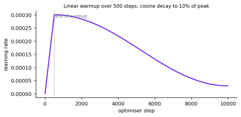
- Weight decay done right. With Adam, adding an L2 penalty to the loss is not the same as decaying the weights; AdamW (1711.05101) decouples the two, which is what large runs use.
- Gradient clipping. Rescaling the gradient when its overall norm exceeds a threshold (1211.5063) keeps one bad batch from throwing the weights far off.
- Loss spikes and NaNs are the most common failures of long runs. Usual suspects, roughly in order: a bad batch of data, a learning rate too high for the batch size, fp16 overflow, and numerically unstable operations (softmax and normalisation in low precision). Keep checkpoints frequent enough to roll back past a spike, and log the gradient norm, which usually rises before the loss does.
11. How much compute, how long?
Training compute is about floating-point operations for parameters and training tokens (2 per parameter per token forward, 4 backward; 2001.08361). Wall-clock time is that divided by what the GPUs actually deliver:
MFU (model FLOPs utilisation) is the share of peak arithmetic throughput the run achieves; data loading, communication, small kernels and the pipeline bubble keep it well below 1.
Two worked examples with round, hypothetical hardware numbers:
- Total cost. 1 billion parameters on 100 billion tokens is FLOPs. On 8 GPUs with 1,000 TFLOP/s peak each at 40 percent MFU that is about 190,000 seconds, a little over 2 days.
- One step. 8 GPUs × 4 sequences × 4,096 tokens is 131,072 tokens. For a 7B model that is FLOPs, about 1.7 seconds at the same speed. The 0.25 seconds of gradient all-reduce from section 4 fits inside it.
12. Measuring efficiency
Turn the formula around to check a running job: from measured tokens per second, compute the MFU
(model_flops_utilisation, in the schedule code of section 10).
For example, a 7B model processing 3,000 tokens per second per GPU on GPUs with 312 TFLOP/s of bf16 peak is at percent MFU. Typical reasons a run sits far lower, and what to check:
| Symptom | Likely cause | Check |
|---|---|---|
| GPUs idle between steps | Data loading or image decoding | Step time with synthetic data |
| Step time grows with GPU count | Communication not overlapped, slow links | Profile with communication shown |
| Low utilisation, small model | Kernels too small, launch overhead | Larger micro-batch, compiled graph |
| Memory errors at a larger batch | Activations | Checkpointing, sequence or tensor parallelism |
13. A checklist for a first large run
These are standard practices, written as our recommendations:
- Write the memory and compute budget first. Sections 2 and 11 give both in a few lines; the plan should fit before you book GPUs.
- Measure MFU and step time from day one, with and without real data.
- Make it restartable. Checkpoint model, optimiser and data-loader state; large runs lose nodes. Test a restart before the long run, not after the first failure.
- Start from a scaling ladder. Train three or four small models first, fit how the loss falls (Scaling laws and data recipes), and only then spend the big budget.
- Evaluate during training. Closed-loop or held-out metrics on a schedule catch a broken run in hours instead of days.
- Log everything that can change a result: code version, data snapshot, seeds, effective batch size, learning-rate schedule, loss scale and gradient norm.
Reference implementation (PyTorch)
libs/tutorial/training_scale.py; tests are in libs/tutorial/tests/test_training_scale.py. They
check: 16 bytes per parameter for mixed-precision Adam and the ZeRO stage arithmetic; the compute and
wall-clock formulas; data-parallel averaging, gradient accumulation and activation checkpointing all
match the full-batch gradient; the exact activation bytes saved with and without checkpointing, and
that they double with the batch; ring all-reduce sums correctly and sends of the tensor;
the tensor-parallel MLP equals the unsplit layer; the pipeline bubble formula; loss scaling rescues
underflowing gradients until it overflows; the warmup-cosine schedule; and the MFU arithmetic. Run
uv run --group tutorial python -m libs.tutorial.training_scale.
Check yourself
- Why does the backward pass cost about twice the forward pass?
- Where do the 16 bytes per parameter of mixed-precision Adam come from, and which of them does each ZeRO stage shard?
- Why does data parallelism alone not let you train a larger model?
- In a ring all-reduce on GPUs, how much does each GPU send, and why does it hardly depend on ?
- Why does Megatron split the first MLP matrix by columns and the second by rows?
- A pipeline has 8 stages. How many micro-batches keep the bubble under 20 percent?
- Why does fp16 training need loss scaling and bf16 training usually does not?
- A 3B model trains on 300B tokens on 16 GPUs at 1,000 TFLOP/s peak and 40 percent MFU. How many days?
Quiz
Answer each question; feedback appears as soon as you choose.
Sources
- Kingma and Ba, Adam, 2014.
- Rajbhandari et al., ZeRO: Memory Optimizations Toward Training Trillion Parameter Models, 2019.
- Zhao et al., PyTorch FSDP, 2023.
- Shoeybi et al., Megatron-LM, 2019.
- Huang et al., GPipe, 2018.
- Micikevicius et al., Mixed Precision Training, 2017.
- Chen et al., Training Deep Nets with Sublinear Memory Cost, 2016.
- Korthikanti et al., Reducing Activation Recomputation in Large Transformer Models, 2022.
- Goyal et al., Accurate, Large Minibatch SGD: Training ImageNet in 1 Hour, 2017.
- Loshchilov and Hutter, Decoupled Weight Decay Regularization, 2017.
- Pascanu et al., On the difficulty of training Recurrent Neural Networks, 2012.
- Kaplan et al., Scaling Laws for Neural Language Models, 2020.
Co-training and catastrophic forgetting
Why fine-tuning a model on a new task erases the old one, a toy that measures it, and four ways to limit it: mixing old data back in, penalising important weights, small learning rates, and adapters.
Distillation: small, fast students from large teachers
Knowledge distillation with soft targets, feature and policy distillation, on-policy distillation, step distillation for diffusion and flow models, and how driving teams use rule-based and reasoning teachers.