VLA models

How RT-2, OpenVLA, pi0 and SmolVLA turn a vision-language model into a robot policy: the anatomy of a forward pass, how actions come out (measured on an ambiguous instruction), training recipes, and how to diagnose a VLA that fails.

The recipe

Start from a pretrained VLM (the Tokens, ViT and VLMs module). Teach it to output robot actions. Train on robot demonstrations, often mixed with the web-scale vision-language data that gave the VLM its general knowledge. The main design question is how actions come out.

Anatomy of one decision

Follow one control step through a VLA, with the shapes involved:

Cameras to patch features. Each image is cut into patches and encoded by a vision transformer (the Tokens, ViT and VLMs module): a 224 by 224 image with 14 by 14 patches gives 256 patch features. Some VLAs combine two vision encoders (OpenVLA uses DINOv2 and SigLIP features).
Projector. A small network maps the patch features into the language model's embedding space, so they become "image tokens". Compressing them here (SmolVLA keeps 64 per frame) is the main lever on cost, as in the Deploying module.
The language model. Image tokens, the instruction's text tokens and often the robot's state go through the transformer together, so every word can attend to every patch.
Action output. Either the language model keeps generating, now action tokens, or an action expert reads its features and generates a continuous chunk (next section).
De-normalise and execute. Actions are trained in a normalised range; the controller gets them back in joint or Cartesian units, executes part of the chunk, and the loop repeats.

Most of the parameters and compute sit in step 3; most of the design choices that decide whether the robot moves well sit in steps 4 and 5.

Two ways to output actions

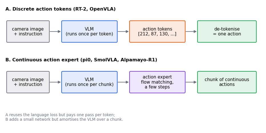
Discrete action tokens. Quantise each action dimension into bins, give the bins token ids, and let the language model generate them like words. Simple, reuses the language head and loss, but sequential and limited by quantisation.
A continuous action expert. Keep the VLM for understanding, and add a smaller network that generates a chunk of continuous actions with flow matching or diffusion (the Diffusion and Flow matching modules), conditioned on the VLM's features. Smooth, fast per chunk, handles multimodality.

Two rows of boxes. Top: image and instruction into a VLM, then action tokens, then de-tokenise to one action. Bottom: image and instruction into a VLM, then a flow-matching action expert, then a chunk of continuous actions. — The two output designs. Discrete tokens run the VLM once per token; an action expert runs the VLM once per chunk and adds a small network that takes a few flow steps.

How actions become tokens

The simplest scheme bins every action dimension at every time step into, say, 256 levels. With a chunk of 50 steps and 7 dimensions that is 350 tokens, and neighbouring tokens are highly correlated, so the sequence is long and redundant. The FAST paper (2501.09747) reports that such per-dimension, per-timestep binning performs poorly on dexterous, high-frequency data. It proposes compressing the action sequence with a discrete cosine transform (a frequency representation, like JPEG for trajectories) and tokenising the coefficients, which gives far fewer tokens per chunk. It also releases a general-purpose tokenizer, FAST+, trained on 1M real robot action trajectories.

The trade-off to remember: tokens keep the VLM's loss and generation machinery but pay in sequence length and quantisation, while a continuous expert pays in an extra network and extra sampling steps. The Tokenizers module measures binning against frequency coding on an action chunk.

Choosing an action head, measured

The head also decides what happens when the right action is ambiguous. The reference code adds a third instruction, "either square", to the mini-VLA scenes below; its demonstrations go to the red or the green square at random. Three heads on the same prefix model:

libs/tutorial/action_heads.py (heads)

class RegressionHead(nn.Module):
    """Pools the prefix and predicts the chunk; trained with squared error."""

    def __init__(self) -> None:
        """Creates the prefix model and an MLP head."""
        super().__init__()
        self.prefix = _Prefix()
        self.head = nn.Sequential(
            nn.Linear(DIM, 4 * DIM), nn.GELU(), nn.Linear(4 * DIM, CHUNK * 2)
        )

    def loss(
        self, images: torch.Tensor, instruction: torch.Tensor, chunk: torch.Tensor
    ) -> torch.Tensor:
        """Mean squared error to the demonstrated chunk."""
        return ((self.act(images, instruction) - chunk) ** 2).mean()

    def act(self, images: torch.Tensor, instruction: torch.Tensor) -> torch.Tensor:
        """The predicted chunk (n, CHUNK, 2): the average of what was demonstrated."""
        pooled = self.prefix(images, instruction).mean(dim=1)
        return self.head(pooled).view(-1, CHUNK, 2)


class BinHead(nn.Module):
    """One categorical over BINS values per coordinate, like parallel action tokens."""

    def __init__(self) -> None:
        """Creates the prefix model and a head with CHUNK * 2 * BINS logits."""
        super().__init__()
        self.prefix = _Prefix()
        self.head = nn.Sequential(
            nn.Linear(DIM, 4 * DIM), nn.GELU(), nn.Linear(4 * DIM, CHUNK * 2 * BINS)
        )

    def _logits(self, images: torch.Tensor, instruction: torch.Tensor) -> torch.Tensor:
        pooled = self.prefix(images, instruction).mean(dim=1)
        return self.head(pooled).view(-1, CHUNK * 2, BINS)

    def loss(
        self, images: torch.Tensor, instruction: torch.Tensor, chunk: torch.Tensor
    ) -> torch.Tensor:
        """Cross-entropy of each coordinate's bin."""
        targets = (
            ((chunk.reshape(len(chunk), -1) + 1) / 2 * BINS).long().clamp(0, BINS - 1)
        )
        return nn.functional.cross_entropy(
            self._logits(images, instruction).transpose(1, 2), targets
        )

    @torch.no_grad()
    def act(self, images: torch.Tensor, instruction: torch.Tensor) -> torch.Tensor:
        """Samples every coordinate's bin independently and returns bin centres."""
        probs = self._logits(images, instruction).softmax(dim=-1)
        bins = torch.multinomial(probs.reshape(-1, BINS), 1).view(
            len(images), CHUNK * 2
        )
        return ((bins.float() + 0.5) / BINS * 2 - 1).view(-1, CHUNK, 2)


class FlowHead(nn.Module):
    """A flow-matching action expert attending to the prefix (as in the mini VLA)."""

    def __init__(self) -> None:
        """Creates the prefix model and the action expert."""
        super().__init__()
        self.prefix = _Prefix()
        self.expert = ActionExpert()

    def loss(
        self, images: torch.Tensor, instruction: torch.Tensor, chunk: torch.Tensor
    ) -> torch.Tensor:
        """Flow-matching loss on the chunk."""
        prefix = self.prefix(images, instruction)
        noise = torch.randn_like(chunk)
        t = torch.rand(len(chunk), 1)
        noisy = (1 - t[:, :, None]) * noise + t[:, :, None] * chunk
        return ((self.expert(noisy, t, prefix) - (chunk - noise)) ** 2).mean()

    @torch.no_grad()
    def act(
        self, images: torch.Tensor, instruction: torch.Tensor, steps: int = 10
    ) -> torch.Tensor:
        """Integrates the expert's flow from noise with Euler steps."""
        prefix = self.prefix(images, instruction)
        chunk = torch.randn(len(images), CHUNK, 2)
        for i in range(steps):
            t = torch.full((len(images), 1), i / steps)
            chunk = chunk + self.expert(chunk, t, prefix) / steps
        return chunk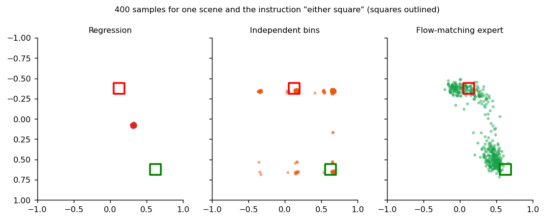

Three scatter plots of 400 sampled endpoints for one scene with the instruction either square. Regression: one tight blob halfway between the two outlined squares. Independent bins: clusters at both squares and at the two mixed corners combining one square's x with the other's y. Flow-matching expert: two clusters, one at each square. — Regression averages the two answers; independently sampled bins pick each coordinate's mode separately and so also produce the two mixed corners; the flow expert picks one square per sample.

Head	Specific instruction: reaches the named square	"Either": reaches one of the squares	"Either": share at the first square
Regression	1.00	0.31 to 0.35	about 0.5
Independent bins	0.99 to 1.00	0.73 to 0.78	about 0.5
Flow-matching expert	0.98 to 0.99	0.84 to 0.94	about 0.5

(Range over 3 seeds, 3,000 training steps; uv run --group tutorial python scripts/tutorial_results.py action_heads. "Reaches" means the final waypoint is within 0.25 of the square, on a scale where the image half-width is 1.) All three are near perfect when the instruction is specific. On the ambiguous one:

Regression lands between the squares, the average of two good answers (the Imitation learning module's obstacle example again).
Independent bins represent each coordinate's two modes correctly but sample them separately, so about half the samples combine one square's x with the other's y. Autoregressive token decoding, as in RT-2 and OpenVLA, avoids this mixing because each token is generated after seeing the ones before it, at the cost of one sequential step per token.
The flow expert samples the whole chunk jointly and picks one square per sample, which is the property pi0 and SmolVLA are after.

For driving, "either" is common: pass the cyclist now or after the oncoming car, merge before or after the truck. A head that averages or mixes those options produces a trajectory nobody would drive.

The models

All facts below are as the papers report.

Model	Backbone	Action output	Notes
RT-2 (2023)	PaLI-X (5B, 55B) or PaLM-E (12B)	Actions as text tokens	Co-fine-tuned on robot and web vision-language data; coined "VLA"; chain-of-thought reasoning added
OpenVLA (2024)	Llama 2 with DINOv2 and SigLIP vision features	Discrete action tokens: each dimension binned into 256 bins between the 1st and 99th percentile of the data, written over the 256 least-used Llama tokens	7B, trained on 970k real robot demonstrations; beats RT-2-X (55B) by 16.5 points in absolute success across 29 tasks; LoRA fine-tuning on consumer GPUs
pi0 (2024)	PaliGemma	Flow-matching action expert	Chunk of 50 actions, 10 integration steps, control up to 50 Hz
SmolVLA (2025)	Compact pretrained VLM	Flow-matching action expert	About 450M parameters; 64 visual tokens per frame; asynchronous inference; trains on one GPU

Alpamayo-R1 (the Driving literature module) is the same family for driving: a reasoning VLM backbone plus a flow-matching expert, with discrete tokens used during training.

Training recipes

The models differ in their heads, but their training follows similar stages:

Start from a pretrained VLM. Its vision and language knowledge comes from web-scale image-text data, which no robot dataset can match.
Robot pretraining on large, mixed demonstration datasets, often from many robots. OpenVLA trains on 970k real robot demonstrations.
Keep the old skills. Training only on robot data tends to erode what the VLM knew; RT-2 co-fine-tunes on robot data together with the original vision-language data, and reports that the result generalises to new objects and instructions.
Fine-tune on the target task and robot, often with LoRA (Efficient fine-tuning and inference) and sometimes with the vision encoder frozen.
Optionally post-train with RL or preferences (RL for alignment); Alpamayo-R1 does this with GRPO.

Two details that matter more than they look:

Action normalisation. OpenVLA bins each dimension between the 1st and 99th percentile of the training data, so rare extreme values do not waste the bins. Get the normalisation wrong between training and deployment and the robot moves at the wrong scale.
Control frequency and chunk length have to match the robot's controller; pi0 predicts 50-step chunks and reports control up to 50 Hz.

Diagnosing a VLA that fails

A VLA has many parts, so a failure needs isolating. Checks in rough order of cost, written as our recommendations:

Check	How	What it tells you
Is the instruction used?	Swap or blank the instruction on held-out scenes	If success does not change, the policy ignores language
Is a simpler policy as good?	Train a small, language-blind baseline on the same data	Whether the VLA's size is helping at all
Can it see the object?	Vary the camera crop or the number of visual tokens	Whether the image tokens are too coarse
Is it the head?	Look at sampled chunks for one scene	Averaging, mixing or jitter point at the action head
Does it run fast enough?	Measure inference and chunk timing on the robot	Stale actions look like a bad policy

Same idea on a robot arm: SmolVLA

On our simulated SO-100 pick-by-colour task (the instruction names the cube), SmolVLA reached 8 to 13 percent with the vision and language parts frozen, and 3 to 7 percent when all parameters were trained. A language-blind ACT baseline reached 16 percent. Our untested hypothesis is that 64 visual tokens are too coarse for a small cube in a wide view; a closer camera would test it.

Take-aways for a learner: a VLA gives you language and general vision features, but it is not automatically better than a small policy, and a failure usually has to be diagnosed, not assumed. Compare against a simple baseline every time.

Reference implementation (PyTorch): a mini VLA

A toy version of the pi0 and SmolVLA structure. A 16 by 16 image holds a red and a green square; the instruction is one token naming a colour; the action is a chunk of 8 waypoints moving from the centre to the instructed square. A prefix model (a tiny ViT plus the instruction token, through transformer blocks) reads the scene once. A small action expert, with cross-attention to the prefix features, predicts the flow-matching velocity of the noisy chunk, and sampling takes ten Euler steps. Tests are in libs/tutorial/tests/test_action_expert.py.

libs/tutorial/action_expert.py (prefix)

class PrefixModel(nn.Module):
    """The "VLM": image patch and instruction tokens through transformer blocks."""

    def __init__(self) -> None:
        """Creates the vision encoder, instruction embedding and joint blocks."""
        super().__init__()
        self.vision = TinyViT(image_size=IMAGE, patch_size=4, dim=DIM, depth=2)
        self.instruction = nn.Embedding(len(COLOURS), DIM)
        self.blocks = nn.ModuleList(TransformerBlock(DIM, heads=4) for _ in range(2))

    def forward(self, images: torch.Tensor, instruction: torch.Tensor) -> torch.Tensor:
        """Returns prefix features (batch, patches + 1, DIM)."""
        tokens = torch.cat(
            [self.vision(images), self.instruction(instruction)[:, None]], dim=1
        )
        for block in self.blocks:
            tokens = block(tokens)
        return tokens

libs/tutorial/action_expert.py (expert)

class ExpertBlock(nn.Module):
    """Self-attention over action tokens, cross-attention to the prefix, an MLP."""

    def __init__(self) -> None:
        """Creates the three sub-layers with their norms."""
        super().__init__()
        self.norm1, self.norm2, self.norm3 = (nn.LayerNorm(DIM) for _ in range(3))
        self.self_attn = MultiHeadAttention(DIM, heads=4)
        self.cross_attn = MultiHeadAttention(DIM, heads=4)
        self.mlp = nn.Sequential(
            nn.Linear(DIM, 4 * DIM), nn.GELU(), nn.Linear(4 * DIM, DIM)
        )

    def forward(self, x: torch.Tensor, prefix: torch.Tensor) -> torch.Tensor:
        """Updates action tokens ``x`` using the prefix features as context."""
        x = x + self.self_attn(self.norm1(x))
        x = x + self.cross_attn(self.norm2(x), context=prefix)
        return x + self.mlp(self.norm3(x))


def time_embedding(t: torch.Tensor, dim: int = DIM) -> torch.Tensor:
    """Sinusoidal embedding of flow time t in [0, 1], shape (batch, dim)."""
    half = dim // 2
    freqs = torch.exp(-math.log(1000.0) * torch.arange(half) / half)
    angles = t * 1000.0 * freqs[None]
    return torch.cat([angles.sin(), angles.cos()], dim=-1)


class ActionExpert(nn.Module):
    """Predicts the flow-matching velocity of a noisy action chunk."""

    def __init__(self) -> None:
        """Creates the input/output projections and two expert blocks."""
        super().__init__()
        self.inp = nn.Linear(2, DIM)
        self.position = nn.Parameter(torch.zeros(1, CHUNK, DIM))
        nn.init.normal_(self.position, std=0.02)
        self.time = nn.Linear(DIM, DIM)
        self.blocks = nn.ModuleList(ExpertBlock() for _ in range(2))
        self.out = nn.Linear(DIM, 2)

    def forward(
        self, noisy: torch.Tensor, t: torch.Tensor, prefix: torch.Tensor
    ) -> torch.Tensor:
        """Maps a noisy chunk (batch, CHUNK, 2) and time (batch, 1) to a velocity."""
        x = self.inp(noisy) + self.position + self.time(time_embedding(t))[:, None]
        for block in self.blocks:
            x = block(x, prefix)
        return self.out(x)

libs/tutorial/action_expert.py (mini_vla)

class MiniVLA(nn.Module):
    """Prefix model plus action expert, trained with a flow-matching loss."""

    def __init__(self) -> None:
        """Creates both parts."""
        super().__init__()
        self.prefix = PrefixModel()
        self.expert = ActionExpert()

    def loss(
        self, images: torch.Tensor, instruction: torch.Tensor, chunk: torch.Tensor
    ) -> torch.Tensor:
        """Flow-matching loss on action chunks, conditioned on the prefix features."""
        prefix = self.prefix(images, instruction)
        noise = torch.randn_like(chunk)
        t = torch.rand(len(chunk), 1)
        noisy = (1 - t[:, :, None]) * noise + t[:, :, None] * chunk
        return ((self.expert(noisy, t, prefix) - (chunk - noise)) ** 2).mean()

    @torch.no_grad()
    def act(
        self, images: torch.Tensor, instruction: torch.Tensor, steps: int = 10
    ) -> torch.Tensor:
        """Runs the prefix once, then integrates the expert's flow with Euler steps."""
        prefix = self.prefix(images, instruction)
        chunk = torch.randn(len(images), CHUNK, 2)
        for i in range(steps):
            t = torch.full((len(images), 1), i / steps)
            chunk = chunk + self.expert(chunk, t, prefix) / steps
        return chunk

Run uv run --group tutorial python -m libs.tutorial.action_expert (about a minute on a laptop CPU). In our run the mean endpoint error was 0.095 on a scale where the image half-width is 1.0, and the predicted endpoint was closer to the instructed square than to the other one in 96 percent of test scenes. This is a toy: it shows the wiring, not what a real VLA achieves.

Check yourself

Name one advantage and one disadvantage of discrete action tokens.
Why does an action expert let the VLM run once per chunk instead of once per action?
What would you expect to change if you gave SmolVLA more visual tokens?
Why compare against a baseline that ignores language?
Why do independently sampled action bins produce invalid actions when the instruction is ambiguous, and how does autoregressive decoding avoid it?
Why do VLA recipes keep training on web vision-language data alongside robot data?
A VLA fails at a new task. List three checks you would run first, and what each would tell you.

Answers

Advantage: they reuse the language model's head, loss and generation code unchanged. Disadvantage: they are quantised and generated one token at a time, so a chunk is a long, slow sequence (350 tokens for 50 steps × 7 dimensions with plain binning).
The expert generates the whole chunk of continuous actions in a few flow steps, conditioned on features the VLM computed once. With discrete tokens the VLM runs once per action token instead.
Our hypothesis is that 64 visual tokens are too coarse for a small cube in a wide view, so more tokens (or a closer camera) should raise success on pick-by-colour. It is untested; the experiment would show whether vision resolution was the bottleneck.
If a policy that never sees the instruction does as well, the VLA is not using language, and its extra size is not helping. In our arm task a language-blind ACT baseline beat SmolVLA.
Each bin is sampled separately, so for an ambiguous instruction one coordinate can come from the left mode and the next from the right, giving an action in neither mode. Autoregressive decoding conditions each token on the ones already chosen, so once the first commits to a mode the rest follow it.
Training on robot data alone erodes what the VLM learned from the web (catastrophic forgetting); mixing the original vision-language data back in keeps it. RT-2 reports the co-fine-tuned model generalises to new objects and instructions.
Swap or blank the instruction (is language used?); train a small language-blind baseline on the same data (is the VLA's size helping?); vary the camera crop or number of visual tokens (can it see the object?). Then look at sampled chunks (is it the head?) and measure timing on the robot (are actions stale?).

Quiz

Answer each question; feedback appears as soon as you choose.

Question 1 of 5

How does RT-2 output robot actions?

Question 2 of 5

What is pi0's action-output design, according to its paper?

Question 3 of 5

Which design choice keeps SmolVLA small and fast?

Question 4 of 5

What did our SO-100 pick-by-colour results suggest?

Question 5 of 5

Why does an action expert let the VLM run once per chunk?

0 of 5 answered

Sources

The four papers in the table.
Pertsch et al., FAST: Efficient Action Tokenization for Vision-Language-Action Models, 2025.
Hugging Face LeRobot documentation for running SmolVLA and ACT in this repository's tooling.

On this page