Flow matching
Learning a velocity field that carries noise to data: the objective, what the network really learns, why paths curve and how reflow straightens them, ODE solvers, conditioning for robot policies, and how it relates to diffusion.
Why this module
Most recent robot and driving policies that output continuous actions (pi0, SmolVLA, Alpamayo-R1's trajectory decoder) generate them with flow matching. It is the simplest member of the diffusion family to train and the fastest to sample from, which matters when the action has to be ready in tens of milliseconds. This module builds it up on a two-cluster toy where the exact answer is known, so every claim can be checked: what the loss asks for, what the network actually learns, why sampling paths bend, how to make them straight, and how many network calls you really need.
Idea
Diffusion corrupts data and learns to denoise. Flow matching skips the noising process and
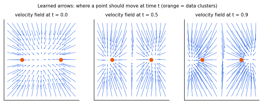
learns directly a velocity field v(x, t): at time t and position x, which way should a point
move so that a cloud of noise samples flows into the data distribution? Sampling is then solving
an ordinary differential equation (ODE), , which you can integrate with a few
Euler steps.
Training
Pair a noise sample x0 ~ N(0, I) with a data sample x1, pick t in [0, 1], and take the
straight-line point between them:
Here is the constant velocity of the straight line from noise to data.
That is the "conditional flow matching" objective with straight paths (also the core of rectified
flow). It is again a plain regression, as simple as diffusion training. The network never sees
which x1 a point was heading to, so at a given (x, t) it learns the average velocity over
all the lines passing through that point.
Sampling
x = noise
for i in range(steps):
    x = x + net(x, t=i/steps) / steps
Exercise: watch the step count matter
Train on two clusters, centred at (-2, 0) and (2, 0), each with standard deviation 0.2:
import torch
from torch import nn

torch.manual_seed(0)
centres = torch.tensor([[-2.0, 0.0], [2.0, 0.0]])


def sample_data(n):
    return centres[torch.randint(0, 2, (n,))] + 0.2 * torch.randn(n, 2)


net = nn.Sequential(nn.Linear(3, 128), nn.SiLU(), nn.Linear(128, 128), nn.SiLU(), nn.Linear(128, 2))
opt = torch.optim.Adam(net.parameters(), lr=1e-3)
for step in range(3000):
    x1 = sample_data(256)
    x0 = torch.randn(256, 2)
    t = torch.rand(256, 1)
    xt = (1 - t) * x0 + t * x1
    loss = ((net(torch.cat([xt, t], dim=1)) - (x1 - x0)) ** 2).mean()
    opt.zero_grad()
    loss.backward()
    opt.step()


@torch.no_grad()
def generate(n, steps):
    x = torch.randn(n, 2)
    for i in range(steps):
        t = torch.full((n, 1), i / steps)
        x = x + net(torch.cat([x, t], dim=1)) / steps
    return x


for steps in (1, 2, 10, 50):
    s = generate(2000, steps)
    d = torch.cdist(s, centres).min(dim=1).values
    print(f"steps={steps:3d} mean distance to nearest mode: {d.mean():.3f}  "
          f"share near right mode: {(s[:, 0] > 0).float().mean():.2f}")
We ran it on CPU (PyTorch 2.7.1, seed 0). Your numbers will differ slightly on other versions:
| Steps | Mean distance to nearest cluster centre | Share on the right cluster |
|---|---|---|
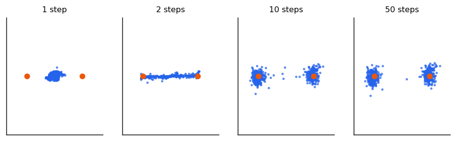
| 1 | 1.746 | 0.44 |
| 2 | 0.960 | 0.51 |
| 10 | 0.268 | 0.53 |
| 50 | 0.256 | 0.52 |
How to read it:
- The data's own spread (std 0.2 in two dimensions) puts a perfect sample about 0.25 from its centre, so 10 and 50 steps are essentially right, and both clusters get about half the samples.
- One step is bad. From noise at
t = 0the network can only output the average velocity over both clusters, which points between them. One Euler step lands in the gap. Several steps let the path commit to one cluster astgrows. - This is the same effect as the "average of two good actions is a bad action" failure in the Diffusion module, now appearing as a step-count effect.
What the network actually learns
The training target depends on which data point the line was heading to, which the network cannot see. So the loss can never reach zero: many lines pass through the same point with different directions, and the best a network can do is predict their average,
This average is the marginal velocity field, and the key result of flow matching (2210.02747) is that following it carries the whole noise distribution exactly onto the data distribution. For the two-cluster toy it has a closed form, because within each cluster the noise, the data point and are jointly Gaussian:
DATA_STD = 0.2


def exact_velocity(x: torch.Tensor, t: torch.Tensor) -> torch.Tensor:
    """The velocity field flow matching converges to, for the two-cluster data.

    With x_t = (1 - t) x0 + t x1, x0 ~ N(0, I) and x1 from cluster k ~ N(mu_k, s^2 I),
    the pair (x_t, x1 - x0) is jointly Gaussian within each cluster, so
    E[x1 - x0 | x_t = x, k] = mu_k + c (x - t mu_k) with c = (t s^2 - (1 - t)) / var_t
    and var_t = t^2 s^2 + (1 - t)^2. The answer is that, averaged over clusters with
    their posterior probabilities given x. This is the "average velocity of all lines
    through x" the training loss regresses onto.
    """
    s2 = DATA_STD**2
    var = t**2 * s2 + (1 - t) ** 2  # (n, 1)
    coeff = (t * s2 - (1 - t)) / var
    means = t[:, None, :] * CENTRES[None]  # (n, k, 2) cluster means of x_t
    sq = ((x[:, None, :] - means) ** 2).sum(dim=-1)  # (n, k)
    weights = torch.softmax(-sq / (2 * var), dim=1)  # posterior over clusters
    per_cluster = CENTRES[None] + coeff[:, None, :] * (x[:, None, :] - means)
    return (weights[..., None] * per_cluster).sum(dim=1)
Two checks, both in the tests:
- The exact field is right. Integrating it with 200 small steps reproduces the data: half the samples on each cluster, each cluster centred at with standard deviation 0.20.
- The network learns the average, not any single line. At the trained network's velocity is within 0.07 (mean squared distance) of the exact field, while the individual training targets scatter 4.5 around it: the loss stays high forever, and that is correct.
| Time | Network vs exact field | Training targets vs exact field |
|---|---|---|
| 0.0 | 0.10 | 4.06 |
| 0.3 | 0.07 | 4.46 |
| 0.6 | 0.14 | 0.85 |
| 0.9 | 0.06 | 1.85 |
(Mean squared distance over 2,000 points; seed 0.) A practical consequence: the training loss tells you little about sample quality, because most of it is this irreducible scatter. Judge a flow model by its samples.
Why paths curve, and how reflow straightens them
Training pairs each noise vector with a random data point, so the straight training lines cross each other everywhere. The learned flow is an ODE, and ODE paths can never cross (each point has one velocity), so the paths bend instead: they start towards the average and then turn towards a cluster. Curved paths are what make a single Euler step land in the gap.
Rectified flow (2209.03003) fixes this with reflow: sample noise, run the trained flow to see where each noise vector actually ends up, and train a new flow on those coupled pairs. The new training lines no longer cross, so the new flow's paths are nearly straight.
def reflow(teacher: VelocityMLP, steps: int = 3000, seed: int = 0) -> VelocityMLP:
    """Rectified flow's reflow: retrain on (noise, sample) pairs the teacher couples.

    Ordinary flow matching pairs noise and data at random, so the straight training
    lines cross and the learned paths curve. Pairing each noise vector with the sample
    the teacher actually carries it to makes the lines non-crossing, and a flow trained
    on them is much straighter.
    """
    torch.manual_seed(seed)
    model = VelocityMLP()
    optimizer = torch.optim.Adam(model.parameters(), lr=1e-3)
    for _ in range(steps):
        x0 = torch.randn(256, 2)
        x1 = euler_sample(teacher, x0, 50)
        t = torch.rand(256, 1)
        x_t = (1 - t) * x0 + t * x1
        loss = ((model(x_t, t) - (x1 - x0)) ** 2).mean()
        optimizer.zero_grad()
        loss.backward()
        optimizer.step()
    return model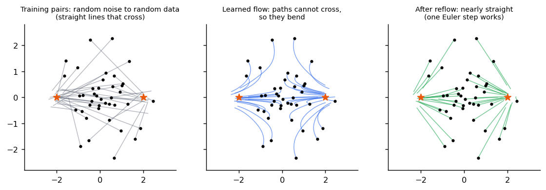
| Model | Path straightness (0 = straight) | Distance to clusters after 1 step | After 2 steps | After 4 steps |
|---|---|---|---|---|
| Learned flow | 1.11 | 1.745 | 0.949 | 0.376 |
| After one reflow | 0.010 | 0.384 | 0.347 | 0.316 |
(A perfect sample is about 0.25 from its centre.) One reflow takes one-step sampling from useless to usable. The price is a second training run, and a little quality: the reflowed flow copies the first flow's mistakes, the same trade as step distillation in the Distillation module.
Solvers: how many network calls?
Sampling is solving an ODE, and Euler's method is the crudest solver: it assumes the velocity stays constant over each step. A midpoint (second-order) step looks ahead half a step and uses the velocity there, at two network calls per step:
@torch.no_grad()
def midpoint_sample(
    velocity: VelocityField, noise: torch.Tensor, steps: int
) -> torch.Tensor:
    """Second-order integration: evaluate the velocity at each step's midpoint.

    Two network calls per step; the error per step falls with the cube of the step
    size instead of the square, so the same budget of calls often goes further.
    """
    x = noise
    h = 1.0 / steps
    for i in range(steps):
        t = torch.full((len(x), 1), i * h)
        x_mid = x + 0.5 * h * velocity(x, t)
        x = x + h * velocity(x_mid, t + 0.5 * h)
    return x


@torch.no_grad()
def path_straightness(
    velocity: VelocityField, noise: torch.Tensor, steps: int = 50
) -> float:
    """Mean squared deviation of the velocity along a path from its average.

    Zero for perfectly straight paths, which one Euler step integrates exactly.
    """
    x, velocities = noise, []
    for i in range(steps):
        t = torch.full((len(x), 1), i / steps)
        v = velocity(x, t)
        velocities.append(v)
        x = x + v / steps
    stacked = torch.stack(velocities)  # (steps, n, 2)
    mean = stacked.mean(dim=0, keepdim=True)
    return ((stacked - mean) ** 2).sum(dim=-1).mean().item()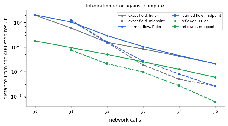
Three lessons for a latency budget (Deploying a driving VLA):
- Count network calls, not steps. A midpoint step costs two.
- With very few calls, Euler is as good as anything; with 8 or more, a second-order solver reaches the same error with fewer calls.
- Straightening the field helps more than a better solver at tiny budgets. The reflowed field with a single Euler call is closer to its converged result than the original field is with four.
Conditioning: from images to action chunks
A policy does not want any sample from the data: it wants an action for this observation. The velocity network simply takes the condition as an extra input, , where is an embedding of the camera images, instruction or route, and the data is an action chunk (the next 50 joint targets, or a trajectory of waypoints). Training and sampling are unchanged.
In VLAs the condition comes from a large vision-language model, and the velocity network is a small action expert that attends to the VLM's features. The VLM runs once per decision; the expert runs the few ODE steps. pi0 (2410.24164) reports 10 integration steps for its action chunk; Alpamayo-R1 uses 5 for its trajectory. A toy action expert with this structure is in the VLA models module.
Flow matching and diffusion
| Diffusion (DDPM-style) | Flow matching (straight paths) | |
|---|---|---|
| Path from noise to data | Set by a noise schedule; curved | Straight line between the pair |
| Network predicts | The added noise (or , or the score) | The velocity |
| Sampling | Stochastic or deterministic (DDIM), often 10 to 1000 steps | ODE, often 5 to 10 steps |
| Loss | Regression | Regression |
They are closer than the table suggests: diffusion's deterministic sampler is also an ODE, and a diffusion model's noise prediction can be converted into a velocity. The practical differences are the path (straight lines are easier to integrate) and the defaults that come with each family. See Diffusion and Sampling and guidance.
Reference implementation (PyTorch)
The exercise above, split into the two functions that matter. Tests are in
libs/tutorial/tests/test_flow_matching.py: the loss is zero for the exact velocity of a single-point
target, one Euler step lands between the clusters and ten do not, both clusters are reached, the
exact field reproduces the data, the network learns the average velocity (and the loss cannot reach
zero), midpoint beats Euler at equal steps, and reflow straightens paths enough for one step. Run
uv run --group tutorial python -m libs.tutorial.flow_matching.
def flow_matching_loss(velocity: VelocityField, x1: torch.Tensor) -> torch.Tensor:
    """Regresses the velocity of the straight line from noise to data.

    Args:
        velocity: A network taking (x_t, t) and returning a velocity of x_t's shape.
        x1: A batch of data points, shape (batch, dim).

    Returns:
        The mean squared error between the predicted and target velocity.
    """
    x0 = torch.randn_like(x1)
    t = torch.rand(len(x1), 1)
    x_t = (1 - t) * x0 + t * x1
    target = x1 - x0
return ((velocity(x_t, t) - target) ** 2).mean()@torch.no_grad()
def euler_sample(
velocity: VelocityField, noise: torch.Tensor, steps: int
) -> torch.Tensor:
"""Integrates dx/dt = v(x, t) from t = 0 (noise) to t = 1 with Euler steps."""
x = noise
for i in range(steps):
t = torch.full((len(x), 1), i / steps)
x = x + velocity(x, t) / steps
return xCheck yourself
- In the exercise, why does one step land between the clusters?
- What does the network see as input, and what does it predict?
- Why is flow-matching training "just regression"?
- Why can the flow-matching loss never reach zero, and what does that mean for using it to judge a model?
- Why do the learned flow's paths curve even though every training line is straight?
- What does reflow train on, and why are its paths straighter?
- A policy needs actions at 10 Hz and each network pass takes 15 ms. How many integration steps fit in the budget if the VLM prefix takes 40 ms?
Quiz
Answer each question; feedback appears as soon as you choose.
Sources
- Lipman et al., Flow Matching for Generative Modeling, 2022.
- Liu et al., Flow Straight and Fast: Rectified Flow, 2022.
- Black et al., pi0, 2024.
- NVIDIA et al., Alpamayo-R1, 2025.
Diffusion
Denoising diffusion models explained step by step: the noise schedule, why predicting noise works, the loss, sampling, and three equivalent views, with figures and code you can check.
Sampling, guidance and diffusion policy
Faster samplers (DDIM and its noise knob, distillation, consistency models), the schedule mismatch that biases deterministic samplers, classifier and classifier-free guidance and what too much guidance does, and diffusion policy over action chunks, with runnable code.