Driving VLA concepts
What a driving vision-language-action model is and how Alpamayo-R1 builds one.
Where details live
This page is the short version. Sensors, data and labels, reinforcement learning and the surrounding literature are covered in the tutorial. Paper statements below were checked against the text of the paper's PDF (arXiv v2).
The idea in one paragraph
A classic driving stack is a pipeline: perception, prediction, planning, control, each with its own interface. An end-to-end model maps camera input (plus the vehicle's own motion history) straight to a future trajectory. A VLA model does that with a pretrained vision-language model (VLM) as the backbone, so it inherits broad world knowledge and can also produce text such as a reasoning trace. The bet is that reasoning about why an action is right helps in rare, ambiguous situations (the long tail) where pure pattern matching is weakest.
Alpamayo-R1 at a glance
Source: Alpamayo-R1, arXiv 2511.00088.
| Part | What the paper describes |
|---|---|
| Backbone | A Cosmos-Reason VLM, a model pretrained for physical-world reasoning (paper) |
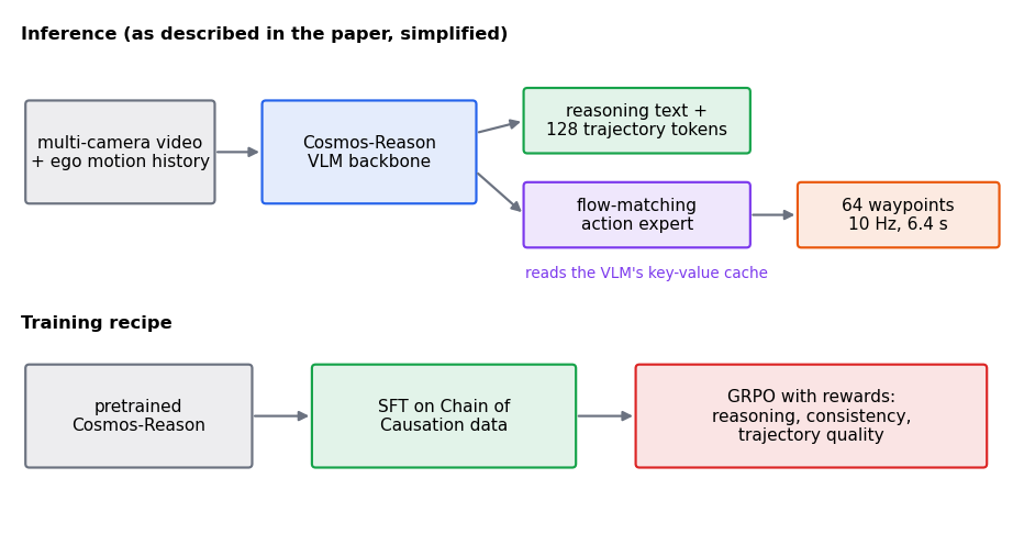
| Input | Multi-camera, multi-timestep observations and the vehicle's recent motion; a 2 s history predicts a 6 s future |
| Output | Reasoning text, then 64 waypoints at 10 Hz (6.4 s) |
| Trajectory form | Unicycle controls (an acceleration and a curvature per waypoint), quantised to 128 discrete tokens that the VLM generates after its reasoning |
| Action expert | At inference, a flow-matching decoder turns those tokens into continuous waypoints, conditioned on the reasoning; trained with a conditional flow-matching loss, Euler steps of 0.1 by default (Sec. 5.1) |
| Data | Chain of Causation (CoC) labels that tie a driving decision to its cause (data module) |
| Training | Supervised fine-tuning, then reinforcement learning with GRPO (RL module) |
Why each choice exists
Chain of Causation labels. Free-form "explain the scene" text tends to describe without deciding. CoC labels tie a decision to the observed cause ("slowing because a pedestrian is about to enter the crosswalk"), so the reasoning is something the action can depend on. Part of the labeling is automatic and part is human-verified; see the data module.
Unicycle controls. Predicting acceleration and curvature gives trajectories a vehicle can follow. Free x, y points do not guarantee that. It is the same reason joint targets are often easier for an arm than free end-effector paths.
Tokens in training, flow matching at inference. The VLM is trained with a next-token loss over the reasoning and the discrete trajectory tokens (so one model does both). At inference a separate flow-matching expert, which reads the VLM's key-value cache, produces smooth continuous waypoints faster than generating tokens. The abstract calls the decoder "diffusion-based", the introduction "diffusion-based ... built on flow matching", and Sec. 5.1 specifies a conditional flow-matching loss, so "diffusion" is used loosely. The paper's latency table (one RTX 6000 Pro Blackwell) breaks 99 ms down as 3.43 ms vision encoder, 16.54 ms prefilling, 70 ms to decode 40 reasoning tokens and 8.75 ms for 5 flow steps; generating the trajectory as 127 tokens instead would take 222 ms and raise the total to 312 ms. A trajectory-only baseline takes 29 ms.
Reasoning. How chain-of-thought-style reasoning is trained, checked and paid for in latency is in the reasoning module.
Reinforcement learning after SFT. Imitation copies the data, including its mistakes. RL optimises a reward directly. The paper combines a reasoning-quality reward, a reasoning-action consistency reward and a trajectory-quality reward.
A latency budget you can check by hand
The paper's latency numbers fit a simple model, which is a useful habit for reading any systems table. Add the stages of the flow-matching path: 3.43 ms (vision encoder) + 16.54 ms (prefill) + 70 ms (decode 40 reasoning tokens) + 8.75 ms (5 flow steps) = 98.7 ms, the 99 ms in the table. The decoding stage is 70 ms for 40 tokens, about 1.75 ms per token. The token route decodes 127 trajectory tokens instead of running the flow expert: 127 × 1.75 ≈ 222 ms, and 3.43 + 16.54 + 70 + 222 ≈ 312 ms, the other number in the table. Two lessons follow.
- Autoregressive decoding costs per token. Cost scales with the number of tokens generated, so a short trajectory code or a parallel decoder (flow matching) is a latency decision as much as a quality one. The efficiency module covers why decoding is limited by memory bandwidth rather than arithmetic.
- Reasoning is the other big line item. 40 reasoning tokens cost 70 ms, more than every other stage together. Longer reasoning would cost 1.75 ms for each extra token on this GPU, which is why the paper lists on-demand reasoning as future work.
Reading it as a modular-stack engineer
If you come from a perception, prediction and planning stack, the table below is our mapping of where each old responsibility goes. It is an interpretation, not the paper's claim, and the right column is where the mapping is weakest.
| Modular stack | In a driving VLA | What you lose or must re-solve |
|---|---|---|
| Perception outputs (boxes, lanes, lights) | Implicit in the backbone's features; critical objects appear in reasoning text | A typed, inspectable interface between components |
| Prediction of other agents | Implicit in the model; the reasoning may name what other agents will do | A separate prediction metric you can test alone |
| Planning with costs and constraints | Generated trajectory, tuned by rewards in RL | Hard constraints; a cost term is a preference, not a guarantee |
| Controls and vehicle limits | Unicycle controls as the output space | Little; this part carries over directly |
| Interface contracts between teams | One model trained end to end | Clear ownership of failures. The bridging module discusses this |
Five questions to ask of any driving VLA paper
- What is the input window and the output horizon? Here, 2 s in and 6 s out (6.4 s of waypoints).
- What does the output space guarantee? Controls give feasibility; tokens give a discrete vocabulary; neither gives collision-freedom.
- Where do the labels come from, and who checked them? See the data module.
- Is the headline metric open loop or closed loop, and how many scenarios? Here, 75 scenarios for the closed-loop ablation, and the error bars matter.
- Is what was released the thing that was measured? The repository FAQ says it is not RL post-trained.
What it measured
- minADE6. The distance between the logged future path and the best of six predicted paths, over the 6.4 s horizon. Open loop.
- Close-encounter rate. The percentage of scenarios where the ego vehicle has a close encounter with another traffic agent. Measured in closed loop in the AlpaSim simulator.
- Closed loop. On a 75-scenario ablation set (Table 8) close encounters fall from 17.0 percent (plus or minus 3.0) to 11.0 percent (plus or minus 2.0) against a trajectory-only baseline, and the AlpaSim score rises from 0.38 to 0.50. Off-road rate does not improve (3.0 percent against 4.0), and the at-fault close-encounter rates (6.0 and 5.0 percent) are within the stated error bars. A 920-scenario public benchmark (Table 10) compares the 10B model with a 0.5B model.
Limits to keep in mind
The paper has no dedicated limitations section. Its future-work section says the current architecture generates reasoning for every input (proposing on-demand reasoning), mentions hierarchical policies, self-supervised auxiliary tasks and world-model integration, and acknowledges the 75-scenario closed-loop set may look small. The points below are our reading, not the authors' claims.
- Open loop is not driving. Matching a logged trajectory says little about what happens when the model's own small errors accumulate. Closed-loop evaluation exists for this reason.
- Auto-generated labels carry the labeler's mistakes. Measure them against a human-verified set.
- Reasoning is not guaranteed to be grounded. A fluent explanation does not prove the model looked at the right thing.
- Released is not the same as published. The public repository ships the 10B weights and inference code. Its FAQ says the released model was not RL post-trained, and that route conditioning and general question answering are not included. The repository is in limited maintenance and points to a newer 1.5 release. Check the model card before assuming a paper result applies to the weights you download.
How this connects to arms
The structure is the one we use in the SO-100 track: a policy that outputs a chunk of future actions, trained on demonstrations, evaluated closed loop.
| Driving (paper) | Arm (our runs) |
|---|---|
| 64-waypoint horizon | Action chunk length. We measured that chunk length was about half of why our reach policy failed |
| Open-loop versus closed-loop gap | We judge policies by closed-loop success rate in simulation, not by training loss |
| Label quality | Demonstrations from a scripted expert are clean, so a policy never sees recovery; we added disturbed demonstrations |
| Language and vision backbone | SmolVLA with an instruction. We measured 8 to 13 percent on pick-by-colour; the cause is not established |
The last row matters: a VLA is not automatically better. In our setup a small VLA did worse than a state-based ACT policy, and we have only a hypothesis (too few visual tokens) for why.
Check yourself
- What does Alpamayo-R1 output, in what order, and which part produces the waypoints at inference?
- Why does the paper predict acceleration and curvature rather than positions?
- Add the four latency stages from the paper's table. Where does the 312 ms of the token route come from?
- On the 75-scenario closed-loop set, which improvements are larger than the stated error bars, and which are not?
- Name two ways the released model differs from the one the paper evaluates.
Answers
- Reasoning text first, then the trajectory. In training the VLM generates 128 discrete trajectory tokens after its reasoning; at inference a flow-matching action expert reading the VLM's key-value cache produces 64 waypoints at 10 Hz (6.4 s).
- Trajectories built from acceleration and curvature are ones a vehicle can follow; free (x, y) points do not guarantee that, and the authors report raw waypoints were hurt by sensor noise.
- 3.43 + 16.54 + 70 + 8.75 = 98.7 ms. Decoding costs about 1.75 ms per token (70 ms for 40 reasoning tokens), so decoding 127 trajectory tokens instead of 5 flow steps takes about 222 ms, giving about 312 ms.
- Close encounters fell from 17.0 ± 3.0 to 11.0 ± 2.0 percent and the AlpaSim score rose from 0.38 to 0.50. The off-road rate did not improve (3.0 against 4.0 percent), and the at-fault close-encounter rates (6.0 and 5.0 percent) are within the error bars.
- The repository FAQ says the released model was not RL post-trained, and that route conditioning and general question answering are not included.
Quiz
Answer each question; feedback appears as soon as you choose.
Driving VLA literature
A guided review of the papers that led to Alpamayo-R1, from modular stacks to reasoning VLAs.
Reading the Alpamayo-R1 code
A guided walk through NVIDIA's released Alpamayo-R1 inference code: the prompt, the trajectory tokens, reasoning generation, the action expert reading the reasoning model's cache, flow-matching sampling and the unicycle action space, with small CPU versions you can run.