Reinforcement learning for policies and reasoning
Policy gradients in depth: the advantage and GAE bias-variance dial, PPO's clip and KL penalty (three estimators compared), GRPO's group baseline and its subtle shrinkage, reward design in Alpamayo-R1, and reward hacking.
Why RL after imitation
New to RL? Start with Reinforcement learning from scratch, which builds up the vocabulary used here (state, reward, return, value, baseline) on a small grid world.
Behaviour cloning (the Imitation learning module) copies the data, mistakes included, and never sees the consequences of its own actions. Reinforcement learning (RL) optimises an outcome directly: the policy acts, a reward scores the result, and the policy changes to make high-reward behaviour more likely. Recent language and driving models use both in sequence: supervised fine-tuning (SFT) first, so the model is competent, then RL to improve what imitation cannot.
The policy gradient idea
A policy gives a probability to each action. After sampling an action and observing its reward:
- if the reward is better than expected, make that action more likely;
- if worse, make it less likely.
The update direction for one sample is
where is the policy and is the advantage. The advantage is the reward minus a baseline (what you expected). Without a baseline the gradient is correct on average but very noisy. The whole family of methods below differs mainly in how they obtain the baseline and how they keep updates safe.
Estimating the advantage: GAE
PPO uses a learned value network (critic) to turn rewards into advantages. The one-step estimate uses the critic's guess of the next state, ; the full Monte Carlo estimate uses every real reward until the end. Generalized Advantage Estimation (1506.02438) blends them with a dial :
is the one-step estimate: low variance, but only as good as the critic. is the Monte Carlo return minus : unbiased, but it accumulates the noise of every step. The reference code measures both on a chain of 20 steps with noisy rewards and a critic that is wrong in the middle:
def gae(
    rewards: torch.Tensor,
    values: torch.Tensor,
    gamma: float = 0.99,
    lam: float = 0.95,
) -> torch.Tensor:
    """Generalized advantage estimation along one episode.

    delta_t = r_t + gamma V(s_t+1) - V(s_t) is the one-step TD error. The advantage
    is the discounted sum A_t = sum_k (gamma lam)^k delta_t+k. With lam = 0 it is the
    one-step estimate (low variance, biased by the critic's errors); with lam = 1 it is
    the full Monte Carlo return minus V(s_t) (unbiased, high variance).

    Args:
        rewards: Shape (T,).
        values: Critic values V(s_0 ... s_T), shape (T + 1,); V(s_T) is 0 at a terminal.
    """
    deltas = rewards + gamma * values[1:] - values[:-1]
    advantages = torch.zeros_like(rewards)
    running = 0.0
    for t in reversed(range(len(rewards))):
        running = deltas[t] + gamma * lam * running
        advantages[t] = running
    return advantages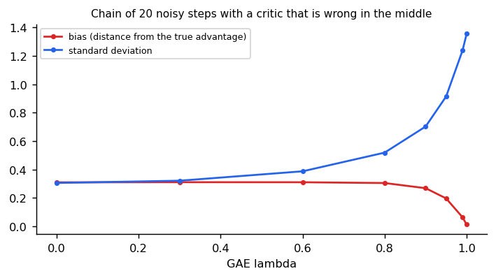
| Bias | Standard deviation | |
|---|---|---|
| 0 | −0.31 | 0.31 |
| 0.9 | −0.27 | 0.70 |
| 0.99 | −0.06 | 1.24 |
| 1 | −0.01 | 1.36 |
Typical practice is around 0.95: enough bootstrapping to tame the variance, enough real reward to wash out most critic error. The cost of all this is the critic itself: another network that must be trained and held in memory, and whose mistakes feed into the policy's gradient.
PPO
Proximal Policy Optimization keeps each update small by clipping the ratio between the new and old action probabilities, so one lucky batch cannot move the policy far. It estimates the baseline with a learned value network (a critic), which is another model to train and store.
What the clip does
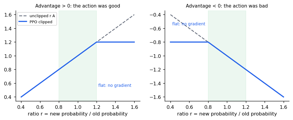
Let and the advantage. The objective for one sample is :
def ppo_objective(
    ratio: torch.Tensor, advantage: torch.Tensor, clip: float = 0.2
) -> torch.Tensor:
    """PPO's clipped surrogate: min(r A, clip(r, 1 - eps, 1 + eps) A)."""
    return torch.minimum(ratio * advantage, ratio.clamp(1 - clip, 1 + clip) * advantage)


def clip_gradient_is_nonzero(ratio: float, advantage: float, clip: float = 0.2) -> bool:
    """Whether the clipped surrogate still has a gradient in the ratio.

    With a positive advantage the gradient is cut once the ratio exceeds 1 + eps (the
    action is already more likely enough); with a negative one, once it falls below
    1 - eps. In the other direction the gradient stays, so a bad step can be undone.
    """
    r = torch.tensor(ratio, requires_grad=True)
    ppo_objective(r, torch.tensor(advantage), clip).backward()
    return bool(r.grad != 0)
Read the plot as a rule: you may make a good action more likely, but only up to 20 percent more likely per update; you may make a bad action less likely, but only down to 80 percent. The gradient vanishes only when the update has already moved far enough in the helpful direction. A test checks all four cases: positive advantage with has no gradient, with it does (the policy made a good action less likely, so it is allowed to repair that); the mirror holds for negative advantage. This is a trust region enforced by a clamp, not by an explicit constraint.
PPO usually runs several epochs of mini-batch updates on each batch of rollouts. The clip is what makes that safe: after a few updates most ratios have left the band and stop contributing.
Penalising drift from a reference: the KL term
For language and driving models the policy must also stay near a reference (the SFT model), or it exploits the reward model (RL for alignment). The penalty is , but with a language model you can only sample from , so it is estimated from the sampled sequence. Three common single-sample estimators, with at the sample:
| Estimator | Formula | Unbiased | Variance | Always |
|---|---|---|---|---|
| k1 | yes | high | no | |
| k2 | no | low | yes | |
| k3 | yes | low | yes |
def kl_estimators(
    logp: torch.Tensor, ref_logp: torch.Tensor
) -> dict[str, torch.Tensor]:
    """Three single-sample estimators of KL(pi || ref) from samples x ~ pi.

    With r = ref(x) / pi(x):

    * k1 = -log r: unbiased, high variance, can be negative;
    * k2 = (log r)^2 / 2: biased, low variance, always non-negative;
    * k3 = (r - 1) - log r: unbiased, low variance, always non-negative (used in GRPO).
    """
    log_ratio = ref_logp - logp
    return {
        "k1": -log_ratio,
        "k2": 0.5 * log_ratio**2,
        "k3": log_ratio.exp() - 1 - log_ratio,
    }
For two three-outcome distributions the true KL is 0.0877; over 200,000 samples k1 averages 0.0877 with standard deviation 0.405, k2 averages 0.0858 (biased) with 0.055, and k3 averages 0.0877 with 0.074. k3 is the best of both, which is why GRPO uses it (its loss code is below). The estimator matters because the penalty's gradient is what trains the model, and a noisy or negative estimate makes training erratic.
GRPO
Group Relative Policy Optimization, introduced in the DeepSeekMath paper, removes the critic. For each prompt it samples a group of outputs, scores each, and uses the group itself as the baseline: the advantage of an output is its reward compared with the group's average (often divided by the group's standard deviation). Fewer models in memory, which matters for large language and vision-language models.
For each prompt, sample outputs with rewards and compute
Then raise the probability of outputs with positive advantage and lower the others, while staying close to a reference model.
A subtle shrinkage
The group mean includes the output being scored. For a group of , the baseline for output contains of its own reward, which removes that share of its signal. The average gradient is therefore shrunk by : half the true size for , three quarters for , 88 percent for . A leave-one-out baseline (the mean of the other outputs) is unbiased. The reference code measures all of them on the four-armed bandit:
MEANS = torch.tensor([0.2, 0.5, 0.8, 0.3])


def group_gradient_samples(
    group: int, baseline: str, trials: int = 20000, noise: float = 0.3, seed: int = 0
) -> torch.Tensor:
    """Gradient estimates for the best arm's logit with a group baseline.

    A softmax policy over four arms (uniform logits) samples ``group`` arms per trial.
    The estimate is (1 / G) sum_i (R_i - b_i) d log pi(a_i) / d logit_best, with:

    * ``"none"``: b = 0;
    * ``"mean"``: b = the group's mean reward (includes sample i itself);
    * ``"leave_one_out"``: b = the mean of the other G - 1 rewards;
    * ``"true"``: b = the policy's expected reward (not available in practice).

    Returns:
        One estimate per trial, shape (trials,).
    """
    generator = torch.Generator().manual_seed(seed)
    arms = torch.randint(0, 4, (trials, group), generator=generator)
    rewards = MEANS[arms] + noise * torch.randn(trials, group, generator=generator)
    if baseline == "none":
        base = torch.zeros(trials, 1)
    elif baseline == "mean":
        base = rewards.mean(dim=1, keepdim=True)
    elif baseline == "leave_one_out":
        base = (rewards.sum(dim=1, keepdim=True) - rewards) / (group - 1)
    elif baseline == "true":
        base = MEANS.mean().expand(trials, 1)
    else:
        raise ValueError(f"unknown baseline {baseline!r}")
    score = (arms == 2).float() - 0.25  # d log pi(a) / d logit_best for uniform logits
    return ((rewards - base) * score).mean(dim=1)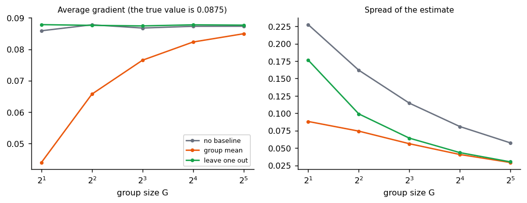
| Group size | No baseline | Group mean | Leave one out |
|---|---|---|---|
| 2 | 0.086 ± 0.227 | 0.044 ± 0.088 | 0.088 ± 0.176 |
| 4 | 0.088 ± 0.162 | 0.066 ± 0.074 | 0.088 ± 0.099 |
| 8 | 0.087 ± 0.115 | 0.077 ± 0.056 | 0.087 ± 0.064 |
| 16 | 0.087 ± 0.081 | 0.082 ± 0.041 | 0.088 ± 0.043 |
(Mean ± standard deviation.) The group mean buys the lowest variance at the price of a slightly shrunk gradient, which Adam's step normalisation largely hides. Leave-one-out keeps the gradient exact and still halves the variance of having no baseline at . Any baseline is far better than none, and larger groups help both; a group of 2 is nearly useless.
Dividing by the group's standard deviation is a separate choice. It makes updates comparable across prompts of different reward scale, but it also inflates prompts where all outputs are nearly equal (a tiny standard deviation makes noise look like signal), which is why the loss code adds a small and why some later variants drop the division.
DeepSeek-R1 showed this style of RL on verifiable rewards (answers that can be checked) can produce long reasoning behaviour. Alpamayo-R1 applies GRPO to a driving VLA.
Exercise: GRPO on a four-armed bandit
Four actions have mean rewards 0.2, 0.5, 0.8 and 0.3, with noise. A softmax policy samples a group of 8 per step and updates with group-normalised advantages. We ran it:
import numpy as np

rng = np.random.default_rng(0)
true_reward = np.array([0.2, 0.5, 0.8, 0.3])  # mean reward of each of four actions
logits = np.zeros(4)
GROUP = 8
LR = 0.5

for step in range(201):
    probs = np.exp(logits) / np.exp(logits).sum()
    actions = rng.choice(4, size=GROUP, p=probs)
    rewards = true_reward[actions] + 0.1 * rng.standard_normal(GROUP)
    advantages = (rewards - rewards.mean()) / (rewards.std() + 1e-8)
    grad = np.zeros(4)
    for action, advantage in zip(actions, advantages):
        onehot = np.eye(4)[action]
        grad += advantage * (onehot - probs)
    logits += LR * grad / GROUP
    if step in (0, 20, 50, 200):
        print(f"step {step:3d}: probabilities {np.round(probs, 2)}")
Output:
step   0: probabilities [0.25 0.25 0.25 0.25]
step  20: probabilities [0.02 0.04 0.91 0.02]
step  50: probabilities [0.   0.01 0.99 0.  ]
step 200: probabilities [0. 0. 1. 0.]
The policy concentrates on the best action (index 2) without any critic.
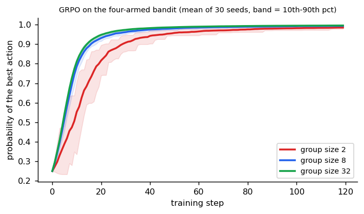
Two experiments to try: make the reward noise larger than the gap between the rewards, and set the group size to 2. The figure suggests learning becomes slower and more variable.
This toy omits the pieces real systems need: a KL penalty to a reference model, clipping, and sampling whole token sequences instead of one action.
Reference implementation (PyTorch)
The same ideas on a toy sequence task: three "prompts", each with a target token sequence, and a
reward equal to the share of matching tokens. The policy is a table of per-position logits so the
code stays about GRPO. Tests are in libs/tutorial/tests/test_grpo.py and include a check that the
clipping stops the gradient for a sample that has already moved far enough; run
uv run --group tutorial python -m libs.tutorial.grpo. The building blocks (GAE, the clip's gradient regions, the
three KL estimators and the group baselines) are in libs/tutorial/policy_gradient.py, with tests
in libs/tutorial/tests/test_policy_gradient.py.
def group_advantages(rewards: torch.Tensor, eps: float = 1e-6) -> torch.Tensor:
    """Scores each output against the other outputs for the same prompt.

    Args:
        rewards: Shape (prompts, group_size).
        eps: Added to the standard deviation so a constant group gives zeros.

    Returns:
        (reward - group mean) / group std, same shape as ``rewards``.
    """
    mean = rewards.mean(dim=1, keepdim=True)
    std = rewards.std(dim=1, keepdim=True)
return (rewards - mean) / (std + eps)def grpo_loss(
logp: torch.Tensor,
old_logp: torch.Tensor,
ref_logp: torch.Tensor,
advantages: torch.Tensor,
clip: float = 0.2,
kl_coef: float = 0.04,
) -> torch.Tensor:
"""Clipped policy-gradient loss with a KL penalty to a reference policy.
All log-probabilities are of whole sampled sequences, shape (prompts, group).
Args:
logp: Log-probability under the policy being trained.
old_logp: Log-probability under the policy that produced the samples.
ref_logp: Log-probability under the frozen reference policy.
advantages: Output of ``group_advantages``.
clip: PPO-style clip range for the probability ratio.
kl_coef: Weight of the KL penalty.
Returns:
A scalar loss to minimise.
"""
ratio = (logp - old_logp).exp()
clipped = ratio.clamp(1 - clip, 1 + clip)
surrogate = torch.minimum(ratio * advantages, clipped * advantages)
# Non-negative estimator of KL(policy || reference) from samples.
delta = ref_logp - logp
kl = delta.exp() - delta - 1
return -(surrogate - kl_coef * kl).mean()def train(
steps: int = 150, group: int = 8, epochs: int = 2, seed: int = 0
) -> list[float]:
"""Runs GRPO and returns the mean reward after each step."""
torch.manual_seed(seed)
policy = TablePolicy(len(TARGETS))
reference = TablePolicy(len(TARGETS))
optimizer = torch.optim.Adam(policy.parameters(), lr=0.1)
history = []
for _ in range(steps):
with torch.no_grad():
sequences = policy.sample(group)
rewards = reward(sequences)
old_logp = policy.log_prob(sequences)
ref_logp = reference.log_prob(sequences)
advantages = group_advantages(rewards)
for _ in range(epochs):
loss = grpo_loss(policy.log_prob(sequences), old_logp, ref_logp, advantages)
optimizer.zero_grad()
loss.backward()
optimizer.step()
history.append(rewards.mean().item())
return historyReward design in Alpamayo-R1
The paper (Sec. 5.3) combines three kinds of reward, checked here against its PDF:
| Reward | How it is computed |
|---|---|
| Reasoning quality | A large reasoning model acts as a critic and scores the reasoning on a 0 to 5 rubric |
| Reasoning-action consistency | Binary: the predicted trajectory is converted to meta-actions and matched with the reasoning by rules; a match scores 1, a mismatch or unparseable text scores 0 |
| Trajectory quality | An L2 error to the expert, a collision indicator and a jerk term, each with a weight |
The paper also adds a safety reward that penalizes unsafe or physically implausible trajectories and reports that it further lowers the close encounter rate. The weights of the terms are not stated. It also describes selecting RL training data where the model's output distribution disagrees most with a reward-based target, mixed with random samples.
Reward hacking
A policy maximises the reward you wrote, not the one you meant. Examples to look for:
- If consistency is rewarded alone, the model can write trivial reasoning that always matches.
- If only collision is penalised, standing still scores well.
- If an LLM critic grades reasoning, the policy may learn to flatter the critic.
That is why the recipe combines several rewards and why evaluation should use a separate closed-loop test, not the training reward.
PPO versus GRPO
| PPO | GRPO | |
|---|---|---|
| Baseline | A learned value network | The group of samples for the same prompt |
| Models in memory | Policy, reference, reward source, critic | Policy, reference, reward source |
| Samples per prompt | One or a few | A group (often 8 to 64) |
| Advantage over time | Per step, with GAE | One per sequence, shared by its steps |
| Works well when | Rewards arrive step by step; a good critic is learnable | A reward is given per whole output; sampling is cheap |
| Main cost | Training and storing the critic | Generating many samples per prompt |
For long language outputs with one end-of-sequence reward, a critic is hard to train and the group is cheap, which is why GRPO took over in reasoning RL. For control problems with dense rewards, PPO's per-step credit assignment remains the better fit.
Check yourself
- Why is a baseline needed in a policy gradient, and what does GRPO use instead of a critic?
- What would you expect if the group size is 2 instead of 8?
- Why do SFT and RL come in that order?
- Give a way a driving policy could exploit a reward based only on collisions.
- What does the PPO clip do when the advantage is positive and the ratio is already 1.3? And when it is 0.7?
- What does lambda control in GAE, and what goes wrong at each extreme?
- Why is the group mean a slightly biased baseline, and what fixes it?
Answers
- Without one, every sampled action is pushed up in proportion to its raw reward, so the gradient is very noisy; subtracting what was expected leaves only how much better or worse the action was. GRPO uses the mean reward of a group of outputs for the same prompt instead of a learned critic.
- A much weaker and noisier signal: the group mean shrinks the gradient to (G − 1)/G, half its size at G = 2, and the estimate is close to useless.
- RL improves on what the policy already does: it needs samples that sometimes earn reward. SFT makes the model competent first, so RL starts from sensible behaviour instead of random outputs.
- Stop, or drive very slowly: a car that never moves never collides. Rewards need progress and comfort terms, and a reference model to stay close to.
- At r = 1.3 with a positive advantage the clipped term is flat (r is above 1.2), so there is no gradient: the action is already 30 percent more likely. At r = 0.7 the unclipped term is the smaller one, so the gradient remains and the update can repair having made a good action less likely.
- It blends the one-step estimate (λ = 0) with the full Monte Carlo return (λ = 1). Small λ trusts the critic, so a wrong critic biases the advantage (bias 0.31 in the toy); large λ trusts the noisy rewards, so variance grows (standard deviation 1.36 at λ = 1).
- The group mean includes the output being scored, so a share 1/G of its own reward is subtracted from its signal. A leave-one-out baseline, the mean of the other G − 1 outputs, is unbiased.
Quiz
Answer each question; feedback appears as soon as you choose.
Sources
- Schulman et al., Proximal Policy Optimization Algorithms, 2017.
- Schulman et al., High-Dimensional Continuous Control Using Generalized Advantage Estimation, 2015.
- Shao et al., DeepSeekMath, 2024 (GRPO).
- DeepSeek-AI, DeepSeek-R1: Incentivizing Reasoning Capability in LLMs via Reinforcement Learning, 2025.
- Ouyang et al., Training language models to follow instructions with human feedback, 2022 (RLHF).
- Alpamayo-R1, arXiv 2511.00088, Sec. 5.3.
Reinforcement learning from scratch
A beginner's path through RL: agents, rewards, returns, values, the Bellman equation, dynamic programming, Monte Carlo and TD learning, Q-learning and SARSA, exploration, DQN and policy gradients, with code you can run.
RL for real robots: sim-to-real
Why policies trained in simulation fail on hardware, and what domain randomization (how wide?), massively parallel training and RMA-style adaptation buy, with a runnable toy, measured trade-offs, and a checklist for driving and robot simulators.