Imitation learning and action chunking
Behaviour cloning, why it drifts (measured on a lane-keeping toy), DART and DAgger, action chunks and temporal ensembling, and why generative policies help, with our SO-100 measurements.
Behaviour cloning
Collect demonstrations as pairs (observation, action) and train a network to predict the action from the observation: supervised learning, exactly like classification or regression. It is the base of nearly every recent robot policy, including driving.
Why it fails: compounding error
Training data comes from the expert's states. At run time the policy makes a small error, lands in a state the expert never visited, errs more there, and drifts. Errors compound over the horizon. DAgger addresses this by having the expert label states the learner visits. A cheaper variant, DART, injects noise into the expert while collecting data so demonstrations contain recoveries.
The problem, measured
A lane-keeping toy makes the mechanism concrete. A car at 5 m/s is nudged by a random heading disturbance every 0.1 s. The expert steers gently near the lane centre and firmly once it is more than 0.3 m off. A small network learns to imitate it from 20 clean demonstrations.
def expert_action(state: torch.Tensor) -> torch.Tensor:
    """The expert's steering: gentle near the lane centre, firm once off by 0.3 m.

    Near the centre it mostly damps the heading; beyond 0.3 m it steers back hard.
    Clean demonstrations rarely leave the gentle zone, so they never show the firm
    correction, which is the point of the toy.
    """
    e, psi = state[..., 0], state[..., 1]
    firm = 3.0 * torch.relu(e.abs() - 0.3) * torch.sign(e)
    return (-2.5 * psi - 0.05 * e - firm).clamp(-1.0, 1.0)


def step(
    state: torch.Tensor, action: torch.Tensor, disturbance: torch.Tensor
) -> torch.Tensor:
    """One time step: heading changes with the action plus a disturbance."""
    e, psi = state[..., 0], state[..., 1]
    e = e + DT * SPEED * torch.sin(psi)
    psi = psi + DT * action + disturbance
    return torch.stack([e, psi], dim=-1)
The trap: clean demonstrations almost never leave the gentle zone (0.15 percent of their states are more than 0.3 m off), so the learner never sees the firm correction. At test time, with somewhat stronger disturbances, it drifts past 0.3 m, does not know to steer back, and keeps drifting.
def collect(
    episodes: int,
    horizon: int,
    *,
    learner: nn.Module | None = None,
    action_noise: float = 0.0,
    disturbance: float = 0.01,
    generator: torch.Generator,
) -> tuple[torch.Tensor, torch.Tensor]:
    """Rolls out and records (state, expert action) pairs.

    Who drives decides which states are seen; the label is always the expert's action:

    * behaviour cloning: the expert drives (``learner`` None, no noise);
    * DART: the expert drives with ``action_noise`` added to what is executed;
    * DAgger: the ``learner`` drives and the expert only labels.
    """
    state = torch.zeros(episodes, 2)
    state[:, 0] = 0.05 * torch.randn(episodes, generator=generator)
    states, labels = [], []
    for _ in range(horizon):
        label = expert_action(state)
        states.append(state)
        labels.append(label)
        if learner is not None:
            with torch.no_grad():
                executed = learner(state).squeeze(-1)
        else:
            executed = label + action_noise * torch.randn(episodes, generator=generator)
        noise = disturbance * torch.randn(episodes, generator=generator)
        state = step(state, executed, noise)
return torch.cat(states), torch.cat(labels)def behaviour_cloning(
seed: int = 0, episodes: int = 20, horizon: int = 100
) -> nn.Module:
"""Fits the learner to clean expert demonstrations."""
generator = torch.Generator().manual_seed(seed)
torch.manual_seed(seed)
learner = _policy()
_fit(learner, *collect(episodes, horizon, generator=generator))
return learner
def dart(
seed: int = 0, episodes: int = 20, horizon: int = 100, noise: float = 0.5
) -> nn.Module:
"""Fits to demonstrations with perturbed executed actions; labels stay clean."""
generator = torch.Generator().manual_seed(seed)
torch.manual_seed(seed)
learner = _policy()
_fit(learner, *collect(episodes, horizon, action_noise=noise, generator=generator))
return learner
def dagger(
seed: int = 0, episodes: int = 20, horizon: int = 100, rounds: int = 4
) -> nn.Module:
"""Starts from behaviour cloning, then repeatedly lets the learner drive and the
expert label the states it reaches, refitting on everything collected so far."""
generator = torch.Generator().manual_seed(seed)
torch.manual_seed(seed)
learner = _policy()
states, labels = collect(episodes, horizon, generator=generator)
_fit(learner, states, labels)
per_round = episodes // rounds
for _ in range(rounds - 1):
new_states, new_labels = collect(
per_round, horizon, learner=learner, disturbance=0.03, generator=generator
)
states, labels = (
torch.cat([states, new_states]),
torch.cat([labels, new_labels]),
)
_fit(learner, states, labels)
return learner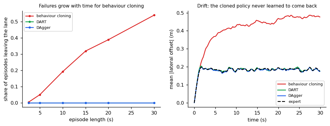
| Episode length | Behaviour cloning leaves the lane | DART | DAgger | Expert |
|---|---|---|---|---|
| 5 s | 5% | 0% | 0% | 0% |
| 10 s | 17 to 22% | 0% | 0% | 0% |
| 15 s | 29 to 36% | 0% | 0% | 0% |
| 30 s | 50 to 59% | 0% | 0% | 0% |
(Range over 3 training seeds.) The failure grows with time because every extra second is another chance to wander into states the demonstrations never covered. Ross, Gordon and Bagnell (1011.0686) put it formally: sequential prediction breaks the i.i.d. assumption of supervised learning, because the policy's own predictions decide what it sees next; their remedy (DAgger) is guaranteed to find a policy that performs well on the distribution of states it induces.
Two fixes: who drives during data collection
| Behaviour cloning | DART | DAgger | |
|---|---|---|---|
| Who drives | The expert | The expert, with noise added to what is executed | The learner |
| Who labels | The expert | The expert (clean command) | The expert, on the learner's states |
| States covered | Only the expert's | The expert's plus nearby disturbances | Wherever the learner goes |
| Cost | Cheapest | One collection pass | Repeated rounds, an expert on call |
DAgger trains, lets the learner drive, asks the expert what it would have done in the states the learner reached, adds those to the data and retrains. DART (1703.09327) gets most of the benefit without letting the learner drive: it injects noise into the expert's executed actions so the demonstrations themselves contain recoveries, while the labels stay the expert's clean commands. Its authors argue that DAgger's on-policy labelling is tedious for human supervisors, and report on a simulated Humanoid task that DART is up to 3 times faster in computation time and that the noise lowers the supervisor's reward during data collection by only 5 percent.
Both fix the toy completely: 0 failures in 30-second episodes for all three seeds. With humans as experts, DART-style collection (deliberately disturb the robot or car, record the human's correction) is usually the practical choice; with a scripted or model expert, DAgger is easy.
Same idea on a robot arm
In our simulated SO-100 arm experiments, a pick-and-place policy trained on clean scripted demonstrations failed. With demonstrations collected under injected disturbance and labelled with the clean plan, success rose from 0 to 94 percent (together with a suitable chunk length).
Action chunking
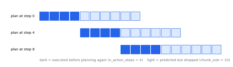
Predict not one action but a chunk of the next k actions, and execute several before
predicting again. Benefits: fewer decisions per second (less compounding), smoother motion, and
the ability to represent a temporally extended intention (a pause, a commitment to one mode).
In LeRobot terms there are two knobs: how many actions the model predicts (chunk_size) and how
many it executes before re-planning (n_action_steps).
Same idea on a robot arm
On our SO-100 reach task, chunk length accounted for about half of the failure, with compounding error the other half. Chunk length is a real hyperparameter, not a detail.
What the chunk length trades
Inside a chunk the policy runs open loop: it does not look at new observations until the chunk ends. That is both the benefit and the risk:
| Longer chunks executed | Shorter chunks executed |
|---|---|
| Fewer decisions, so fewer chances to compound errors | React sooner to surprises |
| Smoother motion, one consistent intention | Can switch intention mid-motion (dithering) |
| Fewer inference calls (latency budget) | More inference calls |
| Blind to disturbances until the chunk ends | Each decision sees fresh, possibly noisy observations |
ACT (Action Chunking with Transformers, 2304.13705) predicts chunks with a transformer and trains with a conditional VAE (the VAE module); the paper reports 80 to 90 percent success on fine bimanual tasks such as slotting a battery, from only 10 minutes of demonstrations. It also uses temporal ensembling: it predicts a new chunk at every step and averages all the predictions that cover the current time step, weighting them with exponentially decaying weights, which smooths execution while still reacting at every step. Diffusion Policy generates the chunk with a diffusion model and uses receding horizon control: predict a chunk, execute the first part, re-predict.
Why generative policies
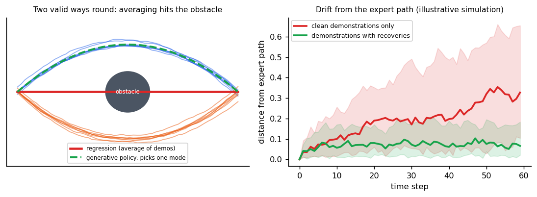
Plain regression averages modes. If the demonstrations go around an obstacle on the left or the right, the average goes into the obstacle. A VAE (ACT) or a diffusion/flow model (Diffusion Policy, pi0) represents the distribution and picks one mode. The same logic applies to driving: at a junction several trajectories are valid, and a good planner should commit to one.
Reference implementation (PyTorch)
The lane-keeping study is libs/tutorial/imitation.py, with tests in
libs/tutorial/tests/test_imitation.py: the expert is gentle near the centre and firm beyond 0.3 m,
clean demonstrations almost never leave the gentle zone while noisy execution reaches the firm zone
far more often, behaviour cloning leaves the lane in more than 30 percent of 30-second episodes and
far more often than in 5-second ones, and DART and DAgger each keep failures under 2 percent. Run
uv run --group tutorial python -m libs.tutorial.imitation.
A second toy makes the point: every demonstration passes an obstacle on the left or the right, and
the observation is the same for both. A regression policy averages the two; an ACT-style
conditional VAE draws a latent that picks a side. Tests are in
libs/tutorial/tests/test_chunked_policy.py; run uv run --group tutorial python -m libs.tutorial.chunked_policy.
The real ACT uses transformers for the encoder and decoder; this version uses MLPs to keep the
idea visible.
class RegressionPolicy(nn.Module):
    """Predicts the whole chunk with one forward pass and a mean-squared-error loss."""

    def __init__(self, hidden: int = 128) -> None:
        """Creates the MLP from an observation to a flattened chunk."""
        super().__init__()
        self.net = nn.Sequential(
            nn.Linear(1, hidden), nn.ReLU(), nn.Linear(hidden, CHUNK * 2)
        )

    def forward(self, obs: torch.Tensor) -> torch.Tensor:
        """Returns a chunk of shape (batch, CHUNK, 2)."""
        return self.net(obs).view(-1, CHUNK, 2)

    def loss(self, obs: torch.Tensor, chunk: torch.Tensor) -> torch.Tensor:
        """Mean squared error to the demonstrated chunk."""
return ((self(obs) - chunk) ** 2).mean()class CvaeChunkPolicy(nn.Module):
"""ACT-style policy: a style latent z explains which demonstration this was.
During training an encoder reads the demonstrated chunk and produces z. The
decoder maps (observation, z) to the chunk. At run time there is no
demonstration to read, so z is drawn from the prior (or set to zero).
"""
def __init__(self, hidden: int = 128) -> None:
"""Creates the encoder and decoder MLPs."""
super().__init__()
self.encoder = nn.Sequential(
nn.Linear(CHUNK * 2, hidden), nn.ReLU(), nn.Linear(hidden, 2 * LATENT)
)
self.decoder = nn.Sequential(
nn.Linear(1 + LATENT, hidden), nn.ReLU(), nn.Linear(hidden, CHUNK * 2)
)
def decode(self, obs: torch.Tensor, z: torch.Tensor) -> torch.Tensor:
"""Maps an observation and a latent to a chunk (batch, CHUNK, 2)."""
return self.decoder(torch.cat([obs, z], dim=-1)).view(-1, CHUNK, 2)
def loss(
self, obs: torch.Tensor, chunk: torch.Tensor, beta: float = 0.05
) -> torch.Tensor:
"""Reconstruction error plus beta times the KL of the latent to N(0, I)."""
mean, log_var = self.encoder(chunk.flatten(1)).chunk(2, dim=-1)
z = mean + torch.exp(0.5 * log_var) * torch.randn_like(mean)
recon = ((self.decode(obs, z) - chunk) ** 2).mean()
kl = (-0.5 * (1 + log_var - mean**2 - log_var.exp()).sum(dim=-1)).mean()
return recon + beta * kl
@torch.no_grad()
def act(self, obs: torch.Tensor, sample_prior: bool = True) -> torch.Tensor:
"""Predicts a chunk with z sampled from the prior, or z = 0 if not sampling."""
shape = (len(obs), LATENT)
z = torch.randn(shape) if sample_prior else torch.zeros(shape)
return self.decode(obs, z)In our test run, the regression policy's paths pass through the obstacle (closest approach 0.21 against an obstacle radius of 0.6), while most latent-sampled paths clear it and both sides are used. Some prior samples still fall between the two modes, so a small share of paths do not clear: the same "holes in the prior" effect as in the VAE module.
Check yourself
- Why do clean expert demonstrations teach nothing about recovery?
- What does DART change in data collection, and why must the label stay the clean command?
- What does a larger chunk length buy and cost?
- Give a driving example where regression to the mean produces an unsafe plan.
- In the lane-keeping toy, why does behaviour cloning get worse as episodes get longer?
- DART and DAgger both fixed the toy. What does each change, and when would you choose which?
- What does temporal ensembling buy over executing one chunk at a time?
Answers
- Clean demonstrations stay near the centre (0.15 percent of their states are more than 0.3 m off), so the learner never sees an off-course state or the correction for it. Once it drifts there at test time it has no data on what to do.
- DART adds noise to the actions the expert executes while collecting, so the car wanders into nearby off-course states. The label stays the expert's clean command so the learner learns the correction, not the noise.
- Longer chunks mean fewer decisions (less compounding), smoother motion with one intention, and fewer inference calls. They cost reaction time: inside a chunk the policy is open loop and blind to disturbances.
- Passing a stopped car: demonstrations go around it on the left or the right, and the average of the two goes straight into it.
- Every extra second is another chance to drift into states the demonstrations never covered. Leaving the lane rose from 5 percent of 5-second episodes to 50 to 59 percent of 30-second ones.
- DART changes the data collection (the expert drives with injected noise) and needs one pass, so it suits human experts. DAgger changes who drives (the learner) and asks the expert to label the learner's states over repeated rounds, which is easy when the expert is a program.
- It predicts a new chunk at every step and averages all predictions covering the current step with decaying weights, so execution is smooth like a chunk while still reacting to new observations every step.
Quiz
Answer each question; feedback appears as soon as you choose.
Sources
- Ross et al., A Reduction of Imitation Learning and Structured Prediction to No-Regret Online Learning, 2010 (DAgger).
- Laskey et al., DART: Noise Injection for Robust Imitation Learning, 2017.
- Zhao et al., ACT / ALOHA, 2023.
- Chi et al., Diffusion Policy, 2023.
Sampling, guidance and diffusion policy
Faster samplers (DDIM and its noise knob, distillation, consistency models), the schedule mismatch that biases deterministic samplers, classifier and classifier-free guidance and what too much guidance does, and diffusion policy over action chunks, with runnable code.
Reinforcement learning from scratch
A beginner's path through RL: agents, rewards, returns, values, the Bellman equation, dynamic programming, Monte Carlo and TD learning, Q-learning and SARSA, exploration, DQN and policy gradients, with code you can run.