Uncertainty and runtime safety
Ensembles, conformal prediction (marginal versus local coverage, and what happens under shift) and runtime monitors (thresholds, false alarms, detection) for deciding when a learned policy should not be trusted, and what the guarantees really cover.
The problem
A learned policy gives an answer for any input, including inputs it has never seen, and it gives it just as fluently. Driving and robot systems need two things beyond accuracy: an estimate of how uncertain a prediction is, and a mechanism that acts on it. Alpamayo-R1's README states the point plainly: the released model is not a complete driving stack and has no redundant safety mechanisms.
Two kinds of uncertainty
- Aleatoric uncertainty is noise in the world that no amount of data removes: a pedestrian may or may not step out, a sensor reading jitters. It is a property of the situation.
- Epistemic uncertainty is the model's ignorance: it has not seen this kind of input. More or better data removes it. It is a property of the model and the data.
They call for different responses. High aleatoric uncertainty says "this is risky even for a perfect model: keep a margin". High epistemic uncertainty says "the model is guessing: do not trust it, ask for help or fall back". An ensemble's disagreement measures the second; a predicted noise level (below) measures the first.
Estimating uncertainty
- Deep ensembles (1612.01474): train several networks from different initialisations and read their disagreement as uncertainty. It is simple and parallelisable, at several times the cost of one model.
- MC dropout (1506.02142): keep dropout on at test time and sample; the authors cast dropout training as approximate Bayesian inference.
In our toy (five small networks trained on a sine curve for inputs in [-2, 2]), the members agree closely inside the data (standard deviation 0.014 at x = 0) and disagree more far outside it (0.053 at x = 5): a warning sign, though a modest one.
Conformal prediction: a guarantee with a condition
A Gentle Introduction to Conformal Prediction and Distribution-Free Uncertainty Quantification (2107.07511) explains the method. For any predictor, hold out a calibration set, record the absolute errors, take the right quantile of them, and use the prediction plus or minus that quantile as an interval:
If calibration and test data are exchangeable (loosely: drawn the same way), the interval contains the truth with probability at least , whatever the model.
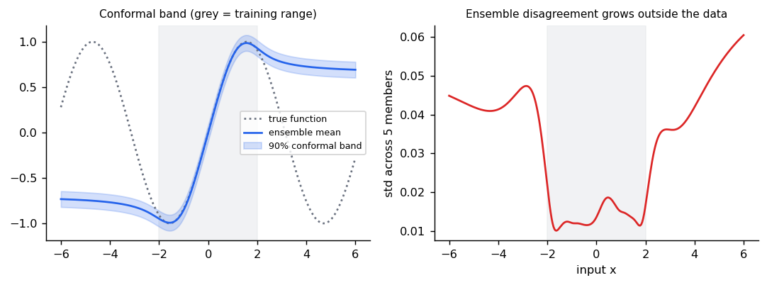
The figure is the important lesson: in our run the conformal half-width was 0.087 and the coverage on fresh data from the same distribution was 0.918 against a target of 0.90. But the band says nothing about inputs from a different distribution. A new town, weather or sensor is exactly the case that matters for driving, so use conformal intervals together with a shift detector, not instead of one.
Intervals that are right on average but wrong where it matters
A conformal guarantee is marginal: averaged over all test inputs, 90 percent are covered. It does not say that each kind of input is covered 90 percent of the time. The toy below has noise that grows with (standard deviation 0.05 at , 0.45 at ), and a constant-width interval calibrated for 90 percent overall.
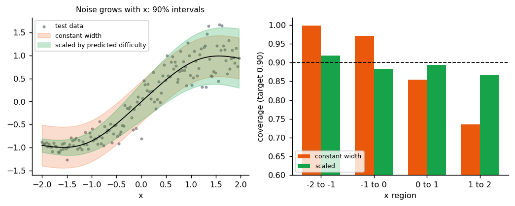
Overall coverage is 0.89, as promised. In the quiet region it is 1.00 (wasteful: wide intervals where a narrow one would do), and in the noisy region only 0.74 (a quarter of the cases miss, exactly where a miss is most costly). The fix is to scale the score by the expected difficulty: train a small model to predict the size of the error at each input, divide the calibration errors by it, take the conformal quantile of the normalised scores, and multiply back at test time:
def noisy_data(
    n: int, low: float = -2.0, high: float = 2.0
) -> tuple[torch.Tensor, torch.Tensor]:
    """y = sin(x) plus noise that grows with x: std 0.05 at x = -2 and 0.45 at x = 2."""
    x = torch.rand(n, 1) * (high - low) + low
    scale = 0.05 + 0.4 * (x + 2) / 4
    return x, x.sin() + scale * torch.randn_like(x)


def fit_scale_model(
    x: torch.Tensor, residual: torch.Tensor, steps: int = 600
) -> nn.Module:
    """Learns the typical size of the error at each input (a "difficulty" estimate)."""
    net = nn.Sequential(nn.Linear(1, 16), nn.Tanh(), nn.Linear(16, 1), nn.Softplus())
    optimizer = torch.optim.Adam(net.parameters(), lr=1e-2)
    for _ in range(steps):
        loss = ((net(x).squeeze(-1) - residual.abs()) ** 2).mean()
        optimizer.zero_grad()
        loss.backward()
        optimizer.step()
    return net


def coverage_by_region(
    lower: torch.Tensor,
    upper: torch.Tensor,
    x: torch.Tensor,
    y: torch.Tensor,
    bins: int = 4,
) -> list[float]:
    """Share of test points inside their interval, in equal-width bins of x."""
    inside = ((y >= lower) & (y <= upper)).squeeze(-1).float()
    edges = torch.linspace(x.min().item(), x.max().item() + 1e-6, bins + 1)
    index = torch.bucketize(x.squeeze(-1), edges[1:-1])
    return [inside[index == k].mean().item() for k in range(bins)]
The scaled intervals are narrow where the data are quiet (width 0.35) and wide where they are noisy (1.21), and coverage in the four regions is 0.92, 0.88, 0.89 and 0.87: closer to uniform, though no longer exactly 0.90 in each, because the guarantee is still only marginal. For driving the lesson is that a headline coverage number hides the rare, hard scenes; check coverage by scenario category (night, rain, dense traffic), as in Evaluating driving models.
When the guarantee stops: distribution shift
Outside the calibration range the guarantee does not merely weaken, it vanishes. In the same toy, for inputs between 2.5 and 3.5 (beyond everything the ensemble and the calibration set saw), the 90 percent interval covered only 34 percent of the truth in our run (a test checks it stays below 50 percent). The ensemble's mean flattens while the sine keeps moving, and the interval keeps its width.
Acting on uncertainty: runtime monitors and safety filters
A monitor does not improve the policy; it decides when not to trust it and hands over to a conservative fallback (stop, slow down, a classical planner).
Choosing the alarm threshold
The simplest monitor raises an alarm when the ensemble's disagreement exceeds a threshold. Setting the threshold is a trade between two errors: false alarms (the fallback triggers on inputs the model handles fine) and missed detections (the policy acts on inputs it should not). Calibrate it on in-distribution data, as a percentile of the disagreement the system sees in normal operation:
def monitor_rates(
    members: list[nn.Module], threshold: float, distance: float, n: int = 2000
) -> tuple[float, float]:
    """False-alarm rate in distribution and detection rate under a shift.

    Alarm when the ensemble's disagreement exceeds ``threshold``. In-distribution inputs
    are drawn from [-2, 2]; shifted ones from a strip of width 0.25 that starts
    ``distance`` beyond the training range, at x = 2 + distance.

    Returns:
        (share of in-distribution inputs flagged, share of shifted inputs flagged).
    """
    x_in = torch.rand(n, 1) * 4 - 2
    x_out = 2 + distance + 0.25 * torch.rand(n, 1)
    _, std_in = ensemble_predict(members, x_in)
    _, std_out = ensemble_predict(members, x_out)
    return (std_in > threshold).float().mean().item(), (
        std_out > threshold
).float().mean().item()| Threshold (percentile of in-distribution disagreement) | False alarms | Detected at the range's edge (0 to 0.25 beyond) | Detected 0.25 or more beyond |
|---|---|---|---|
| 90th | 11% | 88% | 100% |
| 95th | 4 to 5% | 81% | 100% |
| 99th | 1% | 68% | 100% |
(One seed of 5 networks, 4,000 calibration points.) Two things stand out. Far from the data the ensemble disagrees so strongly that every threshold catches it; the difficult cases are at the edge of the training range, where the error is small but non-zero (0.05 in this toy), and a strict threshold misses a third of them. And the false-alarm rate is a real cost: a monitor that cries wolf 5 percent of the time sends a driving system to its fallback every few seconds. Decide the acceptable false-alarm rate first, set the threshold from it, then measure detection.
A caveat for real systems: ensembles of identical architectures can agree with each other and be wrong together on shifted inputs they extrapolate alike (a toy with a sine curve is the easy case), so pair them with an input-space detector and with checks on the model's outputs, such as the Reasoning module's consistency between a trace and the action.
Designing the fallback
A monitor is only as good as what it hands over to. Questions to settle in advance, for driving and for robots:
-
What is the fallback? A minimal-risk manoeuvre (slow and stop in lane), a rule-based planner, a teleoperator, or a more cautious learned mode. It must be simple enough to verify.
-
Can the fallback always run? It needs its own inputs and compute, independent of the component that failed.
-
How fast is the handover? The monitor's latency plus the fallback's must fit inside the time budget (Deploying a driving VLA).
-
What happens when the alarm clears? Avoid flapping between modes by requiring several clear frames before returning.
-
Control barrier functions (1903.11199) verify and enforce safety inside an optimisation-based controller: the controller picks the action closest to the learned one that keeps the system inside a safe set.
-
Safe learning in robotics (2108.06266) reviews three routes: learning-based control that safely improves, RL that encourages safety or robustness, and methods that formally certify a learned policy's safety.
Reference implementation (PyTorch)
Tests are in libs/tutorial/tests/test_conformal.py. They include coverage within three points of
90 percent for a deliberately poor model on exchangeable data, an infinite interval when there are
too few calibration points, and ensemble disagreement more than doubling outside the training
range. Run uv run --group tutorial python -m libs.tutorial.conformal.
def conformal_quantile(scores: torch.Tensor, alpha: float) -> float:
    """The calibration-score quantile that gives 1 - alpha coverage.

    Args:
        scores: Nonconformity scores (for regression, absolute errors) on held-out
            calibration data, shape (n,).
        alpha: Allowed miss rate; 0.1 aims for 90 percent coverage.

    Returns:
        The ceil((n + 1)(1 - alpha))-th smallest score, or infinity when there are too
        few calibration points for that level.

    Raises:
        ValueError: If ``alpha`` is not in (0, 1).
    """
    if not 0.0 < alpha < 1.0:
        raise ValueError(f"alpha must be in (0, 1), got {alpha}")
    n = len(scores)
    rank = math.ceil((n + 1) * (1 - alpha))
    if rank > n:
        return math.inf
    return scores.sort().values[rank - 1].item()


def prediction_interval(
    prediction: torch.Tensor, quantile: float
) -> tuple[torch.Tensor, torch.Tensor]:
    """Lower and upper bounds: the prediction plus or minus the conformal quantile."""
return prediction - quantile, prediction + quantiledef train_ensemble(size: int = 5, steps: int = 800, seed: int = 0) -> list[nn.Module]:
"""Trains ``size`` independently initialised nets on y = sin(x) for x in [-2, 2]."""
members = []
for index in range(size):
torch.manual_seed(seed + index)
net = nn.Sequential(
nn.Linear(1, 32), nn.Tanh(), nn.Linear(32, 32), nn.Tanh(), nn.Linear(32, 1)
)
optimizer = torch.optim.Adam(net.parameters(), lr=1e-2)
for _ in range(steps):
x = torch.rand(128, 1) * 4 - 2
loss = ((net(x) - (x.sin() + 0.05 * torch.randn_like(x))) ** 2).mean()
optimizer.zero_grad()
loss.backward()
optimizer.step()
members.append(net)
return members
@torch.no_grad()
def ensemble_predict(
members: list[nn.Module], x: torch.Tensor
) -> tuple[torch.Tensor, torch.Tensor]:
"""Mean prediction and the members' disagreement (standard deviation)."""
predictions = torch.stack([member(x) for member in members])
return predictions.mean(dim=0), predictions.std(dim=0)def monitored_action(
action: torch.Tensor,
fallback: torch.Tensor,
uncertainty: float,
threshold: float,
) -> torch.Tensor:
"""Uses the learned policy's action unless its uncertainty is too high.
A runtime monitor does not make the policy better; it decides when not to trust it
and hands control to a conservative fallback (stop, slow down, a classical planner).
"""
return fallback if uncertainty > threshold else actionCheck yourself
- What assumption does conformal coverage depend on, and when does it fail?
- Why can a model be wrong and its conformal band still be narrow?
- What does a runtime monitor add that an accurate policy does not give you?
- Name two sources of disagreement in an ensemble and one limit of reading it as uncertainty.
- What is the difference between aleatoric and epistemic uncertainty, and how should a system respond to each?
- A conformal interval has 90 percent coverage overall. Why can it still miss a quarter of the hard cases, and how does scaling the score fix it?
- How would you set a monitor's threshold, and why are the edges of the training range the hard cases?
Answers
- Exchangeability: calibration and test data drawn the same way. It fails under distribution shift, such as a new town, weather or sensor; in the toy, inputs beyond the calibration range were covered only 34 percent of the time.
- The interval width comes from errors on calibration data. On inputs unlike that data the model can be badly wrong while the interval keeps the same width.
- A decision about when not to trust the policy, and a handover to a conservative fallback. Accuracy on the test set does not tell you which inputs the policy is about to get wrong.
- Different initialisations and different minibatch orders (and, in practice, different data subsets). The limit: networks of the same architecture can agree with each other and still be wrong together on shifted inputs.
- Aleatoric is noise in the world that more data cannot remove; respond with margins. Epistemic is the model's ignorance of an input it has not seen; respond by not trusting it: fall back or ask for help.
- The guarantee is marginal: averaged over all inputs. With noise that varies, a constant width over-covers quiet inputs and under-covers noisy ones (0.74 in the noisy region of the toy). Scaling the score by a predicted error size makes intervals wide where the data are noisy, bringing each region near 0.9.
- Choose the acceptable false-alarm rate first, set the threshold as that percentile of in-distribution disagreement, then measure detection. Inputs far outside the data produce large disagreement and are always caught; at the edge the error is small but real and the disagreement barely rises, so a strict threshold misses a third of them.
Quiz
Answer each question; feedback appears as soon as you choose.
Sources
- Angelopoulos and Bates, A Gentle Introduction to Conformal Prediction, 2021.
- Lakshminarayanan et al., Deep Ensembles, 2016.
- Gal and Ghahramani, Dropout as a Bayesian Approximation, 2015.
- Ames et al., Control Barrier Functions: Theory and Applications, 2019.
- Brunke et al., Safe Learning in Robotics, 2021.
World models
What a world model is, a learned dynamics model you can run (one-step versus rollout training, compounding error, planning inside the model), how latent-imagination agents and video world models differ, and where they meet driving.
Safety engineering for learned drivers
A rule-based safety envelope around a learned policy (the RSS longitudinal rule) and what it costs, how many failure-free miles it takes to show a failure rate, why redundancy helps less than it seems, and how safety cases are built.