State estimation and tracking
How a Kalman filter turns noisy detections into position and velocity, how to tell whether its noise settings are honest, what happens when measurements are missing, and where learned models replace it.
Why a learned driving model still needs this
A detector says "a car, 31.2 m ahead". One frame later it says 30.4 m, then 31.5 m. The car is not teleporting; the measurements are noisy. A planner needs a position and a velocity that are smooth enough to plan with, an honest statement of how sure they are, and something sensible when the detector misses a frame. Producing that is state estimation, and in a modular driving stack it sits between perception and prediction (see From modular stacks to end-to-end).
If you come from that world you already know the Kalman filter. This module rebuilds it small enough to run, and then asks the questions that matter in practice: how do I know the filter is tuned honestly, what does it do when the sensor goes quiet, and what do learned models do instead (or in addition)?
One object on a line
A vehicle moves along a line. Its state is : position and velocity. Between steps of s it keeps its velocity, except that a random acceleration nudges it:
The sensor reports only position, with noise: , . Velocity is never measured. The two numbers you must choose are the strength of the random accelerations (which sets ) and the sensor noise . Everything the filter does follows from them.
The filter in two steps
The filter keeps a mean estimate and a covariance that says how uncertain it is. Each time step has two moves.
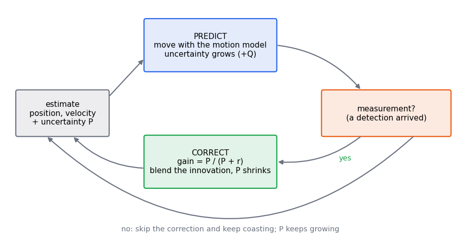
- Predict. Push the estimate through the motion model: , and . Uncertainty grows, because the world may have moved in ways the model did not know.
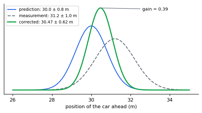
- Correct, if a measurement arrived. Compare the measurement with what the filter expected; the difference is the innovation . Blend it in with a gain that weighs the two sources by how uncertain each is:
When the prediction is very uncertain (large ) the gain is large and the measurement wins; when the sensor is very noisy (large ) the gain is small and the model wins. That is the whole idea.
In the code below the filter also returns the position standard deviation and a statistic called NIS, which we use shortly.
def kalman_filter(
    measured: torch.Tensor,
    accel_std: float,
    meas_std: float,
    missing: torch.Tensor | None = None,
) -> tuple[torch.Tensor, torch.Tensor, torch.Tensor]:
    """Runs a constant-velocity Kalman filter over position measurements.

    Each step predicts with the motion model (the state moves, uncertainty grows by the
    process noise) and then, if a measurement arrived, corrects it (the gain weighs the
    measurement against the prediction by their uncertainties).

    Args:
        measured: Position measurements, shape (n,).
        accel_std: Assumed standard deviation of the random acceleration (m/s^2).
        meas_std: Assumed standard deviation of the position noise (m).
        missing: Optional boolean mask, True where the measurement was lost.

    Returns:
        Estimates (n, 2), position standard deviation (n,) and the normalised innovation
        squared (n,), which is NaN where there was no measurement.
    """
    f = torch.tensor([[1.0, DT], [0.0, 1.0]], dtype=torch.float64)
    g = torch.tensor([0.5 * DT**2, DT], dtype=torch.float64)
    q = accel_std**2 * torch.outer(g, g)
    r = meas_std**2
    x = torch.tensor([measured[0], 0.0], dtype=torch.float64)
    p = torch.diag(torch.tensor([meas_std**2, 100.0], dtype=torch.float64))
    estimates, spreads, nis = [], [], []
    for t in range(len(measured)):
        x = f @ x
        p = f @ p @ f.T + q
        if missing is not None and bool(missing[t]):
            nis.append(torch.tensor(float("nan"), dtype=torch.float64))
        else:
            innovation = measured[t] - x[0]
            s = p[0, 0] + r
            gain = p[:, 0] / s
            x = x + gain * innovation
            p = p - torch.outer(gain, p[0])
            nis.append(innovation**2 / s)
        estimates.append(x)
        spreads.append(p[0, 0].sqrt())
    return torch.stack(estimates), torch.stack(spreads), torch.stack(nis)
What the filter buys you
In our run (a 30 s track, true acceleration noise 1 m/s², true sensor noise 1 m):
| Quantity | Without the filter | With the filter |
|---|---|---|
| Position error (RMSE) | 0.94 m (the raw measurement) | 0.39 m |
| Velocity error (RMSE) | 13.1 m/s (difference of consecutive positions) | 1.3 m/s |
The velocity row is the one to remember. Differencing noisy positions amplifies the noise by , giving a velocity estimate that is useless; the filter infers velocity from the pattern of positions over time and gets it to within about a metre per second without ever measuring it.
Is the filter honest? The innovation test
How do you know and were chosen well? The filter itself gives a check. If its noise settings are right, each innovation should be about as large as the filter expects: its variance is . So the normalised innovation squared, , should average about 1 for a one-dimensional measurement.
def mean_nis(nis: torch.Tensor) -> float:
    """Average normalised innovation squared over steps that had a measurement.

    For a one-dimensional measurement and an honest filter this is close to 1. Well
    above 1 means the filter is overconfident (it is surprised too often); well below 1
    means it is underconfident (its uncertainty is larger than it needs to be).
    """
    return nis[~nis.isnan()].mean().item()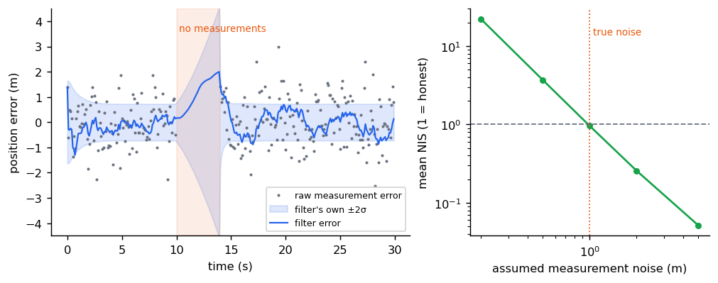
Over five random tracks:
| Filter assumes sensor noise | Mean NIS | Reading |
|---|---|---|
| 0.2 m (too small) | about 22 | Overconfident: it is surprised constantly |
| 1.0 m (true) | 1.0 | Consistent |
| 5.0 m (too large) | 0.05 | Underconfident: its uncertainty is padded |
Two cautions come with this test.
- Consistency is not optimality. With the sensor noise right, the mean NIS was 0.9 to 1.1 for process noises from 0.3 to 3 m/s², a tenfold range, even though position error differed by about 20 percent. NIS can tell you the settings are wrong; it cannot pick the best among settings that are all plausible. For that you need ground truth or a held-out sequence.
- Mean NIS hides structure. A filter can average 1 and still be badly mistuned at the moments that matter (during manoeuvres). Plot NIS over time, and compare it with a chi-square bound, the same way you would check a residual in any regression.
When measurements go missing
Detectors miss objects: occlusion, a bad frame, a sensor dropout. The filter's answer is the predict step alone. In the figure, during a 4 s gap the position standard deviation grows from 0.36 m to 2.3 m. That is the honest outcome: the longer the filter coasts, the less it knows, and downstream code should see that growing , not only the mean. A planner that treats a coasted estimate as precise will drive as if it knew where the car is.
Two design choices follow.
- Track management. After how long a gap do you drop a track? A fixed number of frames is common; a threshold on is more principled, because it measures what you actually know.
- Association. Before a measurement can be used it must be matched to the right track. A wrong match is much worse than a missed one, because it drags the state towards a different object. The gate usually uses the same innovation covariance : accept a detection only if its NIS is below a chi-square threshold. (Matching many detections to many tracks at once is the assignment problem that the DETR module solves with Hungarian matching.)
What the real systems add
The toy has one object, one measured quantity and linear motion. Real stacks extend it.
- Nonlinear models. Vehicles turn. The extended and unscented Kalman filters keep the same predict-correct structure with nonlinear motion and measurement functions; the planning module gives the bicycle model that usually serves as the motion model for a car.
- Ego-motion and time. The estimate must be expressed in a consistent frame while the ego car moves, which is why calibration and time synchronisation matter: a 50 ms timestamp error on a 20 m/s vehicle is a metre of position error that no filter tuning removes.
- Fusion. Radar gives range and velocity directly, cameras give angle and class. Each is just another measurement with its own ; the filter fuses them by correcting in turn.
- Learned components. Networks can predict the measurement noise per detection, replace the motion model, or do the whole tracking step end to end (query-based trackers carry object identities across frames inside the network). The filter's habits remain useful even then: ask the network for an uncertainty, check it for consistency with an NIS-style test, and look at how it behaves when inputs drop out.
Why this matters for a VLA
A driving VLA takes images and returns a trajectory with no explicit tracks. Three things from this module still apply. Time history is information: velocity is not visible in a single frame, which is why these models take a short history of frames and ego motion as input. Dropped inputs happen: test what the model does when a camera freezes, the way you would test a filter over a gap. And the calibration check (is stated confidence matched by behaviour?) is the same question conformal prediction asks of a learned model.
Reference implementation (PyTorch)
Tests are in libs/tutorial/tests/test_state_estimation.py. They check that the filter beats raw
positions and differenced velocity, that honest settings give a mean NIS near one and an
overconfident or underconfident measurement model is flagged, and that uncertainty grows across a
gap and shrinks after it. Run uv run --group tutorial python -m libs.tutorial.state_estimation.
Check yourself
- Why does the covariance grow in the predict step, and what makes it shrink in the correct step?
- A detector reports a position every 0.1 s. Why is velocity from consecutive differences so much worse than the filter's?
- A filter's mean NIS is 20. Which of its settings would you suspect, and in which direction would you change it?
- A filter's mean NIS is 1.0. Does that show its noise settings are the best ones? What would?
- A track loses its detections for 4 s. What should the filter report, and what should a planner do with it?
- Why is a wrong association worse than a missed detection?
Answers
- Predicting pushes the estimate through a motion model that is not exact: the random accelerations it cannot know add Q to the covariance. Correcting with a measurement shrinks it, by an amount set by the gain, which weighs how uncertain the prediction is against how noisy the sensor is.
- Differencing divides measurement noise by the time step, so 1 m of noise at 0.1 s becomes noise of order 10 m/s (13.1 m/s RMSE in the toy). The filter infers velocity from the pattern of many positions through the motion model and reached 1.3 m/s.
- Innovations are about 4.5 times larger than the filter expects, so it is overconfident. Suspect the measurement noise (or the process noise) set too small, and increase it until the mean NIS comes back towards 1.
- No. Several pairs of settings can be equally consistent: in the toy, process noises from 0.3 to 3 all gave a mean NIS between 0.9 and 1.1 while position error differed by about 20 percent. Ranking them needs ground truth or a held-out sequence.
- It should keep predicting and report a growing uncertainty (0.36 m to 2.3 m over 4 s in the toy). A planner should use that uncertainty, for example by keeping a larger margin around the object, and the track manager decides when the track is dropped.
- A missed detection only lets uncertainty grow for a step. A wrong association feeds the track a measurement of a different object, which drags its state, and its velocity, towards the wrong thing. Gating detections by their NIS rejects implausible matches.
Quiz
Answer each question; feedback appears as soon as you choose.
Sources
- Kalman, A New Approach to Linear Filtering and Prediction Problems, Journal of Basic Engineering, 1960, the original filter.
- The toy numbers (position RMSE 0.94 to 0.39 m, velocity 13.1 to 1.3 m/s, NIS 22 / 1.0 / 0.05) are from our reference implementation and are not from any dataset.
Camera geometry and object queries
Coordinate frames, intrinsics and extrinsics, ego-motion compensation, and how DETR-style queries and Hungarian matching turn a set of objects into a loss.
Driving data and labels
Common driving datasets and benchmarks, how labels are produced and checked, and how Alpamayo-R1 builds its reasoning labels.